
CHAPTER 4: Rough Vacuum Regime
4.2 Overview of a Rough Vacuum System
4.3 Gas Load in the Rough Vacuum Regime
4.4.5 Other Rough Vacuum Pumps
4.5.2 Capacitance Diaphragm Gauges
4.5.3 Thermal Conductivity Gauges
4.5.3.3 Thermal Conductivity Gauges and Gas Species Dependencies
4.5.4 Other Rough Vacuum Gauges
4.6 Piping, Valves and Fittings
4.7 Rough Vacuum Pump-Down Process
4.9 Troubleshooting Rough Vacuum Systems
4.9.2 Pump is running, but no vacuum is detected
4.9.3 Deviation from standard pump-down curve
Chapter 4 provides a detailed description of rough vacuum systems and how they function. After you read this chapter, you will be able to:
- Identify the main components present in a rough vacuum system and explain how these components support the function of the system.
- Explain the types of sources that contribute to the gas load in the rough vacuum regime.
- Starting at a specified chamber pressure, calculate intermediate pressures using Boyle’s Law and graph the pump-down curve for a chamber connected to a positive displacement pump based on the respective volumes of the chamber and the pump.
- Describe the principle of operation, applications, maintenance, advantages and limitations of various rough vacuum pumps.
- Describe the principle of operation, applications, maintenance, advantages and limitations of various rough vacuum gauges.
- Calculate the absolute pressure that corresponds to a Bourdon gauge pressure measurement given the atmospheric pressure condition.
- Identify the various types of valves and fittings that are needed to configure a vacuum system.
- Calculate the approximate amount of conductance associated with a cylindrical tube of a specified diameter and length given the gas molecules are moving through it under viscous, laminar flow conditions.
- Calculate an estimated pump-down time for a vacuum system given the volume of the vacuum chamber, the pumping speed of the vacuum pump and the conductance associate with the vacuum piping.
- Explain common vacuum system problems and approaches to troubleshooting these problems.
4.1 Introduction
In the previous chapter, we introduced how a vacuum system functions along with the various underlying components needed to support those functions. In this chapter, we will examine more closely the roughing function, that is, the initial phase of vacuum system operation. During this phase, the vacuum system starts removing the gas load from the chamber. The decreasing pressure level indicates to what extent the gas load is reduced. The starting point for every vacuum system is atmospheric pressure.
Any vacuum system that has been opened to the atmosphere will have a chamber pressure that is equal to the local air pressure conditions. The atmospheric pressure depends upon the elevation and current weather conditions at that specific location. Nominally at sea level, atmospheric pressure is 1 atm, or 760 Torr. When pumped down, the first pressure regime the chamber pressure will pass through is the rough vacuum pressure regime. Sometimes the rough vacuum pressure regime is described as covering a range of pressures from atmosphere to approximately 1 Torr, and the pressure range between 1 Torr to 1 millitorr is called medium vacuum. However, for our discussion, we will define the rough vacuum regime as pressures ranging from 759 Torr to 1 millitorr, about six orders of magnitude for pressure. Over this range, the molecular density of the gas molecules changes from a high of 3 x 10¹⁹ molecules per cubic centimeter (cm3) at 759 Torr to a low of 4 x 10¹³ molecules per cm3 at 1 millitorr. Over the same pressure range, the mean free path of the air molecules increases from 2.5 x 10⁻⁵ mm at 759 Torr to 5.1 cm at 1 millitorr.
This chapter begins with a discussion of the gas load sources starting at the atmospheric pressure condition and through the rough vacuum regime. In the roughing regime, a vacuum system removes the bulk gas, and the pressure in the system drops quickly, provided no gross leaks are present. For vacuum systems operating in a 20°C environment, water vapor present in the gas load can become problematic once the system reaches approximately 20 Torr and poses a challenge for every vacuum system. Good system design, assembly and operating practices lead to more predictable vacuum system performance through the roughing regime.
If a vacuum system is free from gross leaks, the pump-down curve through the roughing regime should be predictable. An estimate of a vacuum system’s pump-down curve through the rough regime can be determined based on the type of mechanical roughing pump selected. A variety of mechanical roughing pumps are available for use in vacuum systems. Each vacuum pump has its advantages and limitations. It is important to understand these differences to properly maintain and service vacuum systems.
A vacuum system needs one or more pressure measurement devices that provide information about how the system is performing. Pressure measurements are taken at regular time intervals after the vacuum system starts its roughing process to generate a pump-down curve. The pump-down curve provides useful diagnostic information to determine the condition of the vacuum system. A variety of pressure measurement devices are available for use in vacuum systems. Just like vacuum pumps, each measurement device has its advantages and limitations. Since the pressure measurement device is often the first indicator checked to assess the operating state of the system, it is important to understand any limitations of the device so the measurement readings are interpreted correctly.
Other hardware components used in a vacuum system impact the vacuum system pump-down time through the roughing regime. Chamber size is important. Increasing the chamber volume and internal surface area increases gas load sources. The tubing and valves used to interconnect the chamber to the vacuum pump should be selected carefully. The conductance that occurs due to the tubing and valves present in the system should not unduly compromise the system’s pump-down performance. And a vacuum system must include a valve that allows at least a part of the system, frequently the chamber, to return to atmospheric pressure conditions so items can be placed in or removed from the system.
After considering the various vacuum system components, we will address the operation of a complete rough vacuum system. This chapter concludes with a short section on troubleshooting rough vacuum systems.
4.2 Overview of a Rough Vacuum System
The components of a rough vacuum system are shown in Figure 4.1. The mechanical roughing pump is capable of reducing the chamber pressure from 760 Torr down to an ultimate pressure near to that specified by the pump manufacturer. A nominal pumping speed in either liters per minute or cubic feet per minute will indicate the rate at which the bulk gas can be evacuated from the chamber. The inlet of the roughing pump is connected to the chamber by tubing or piping. A roughing (isolation) valve is typically placed in the roughing line to provide means of isolating the pump from the chamber by blocking the pathway for the gas to flow between the chamber and the pump. The outlet of the roughing pump is usually connected to the house exhaust system, or if the chamber contains only room air, the exhaust can be left open to the room. The pump should include some type of filter to prevent exhausting particles into the work environment. For example, if an oil-sealed pump is exhausted into a room, then a mist-extractor filter is often attached to the pump’s exhaust fitting.
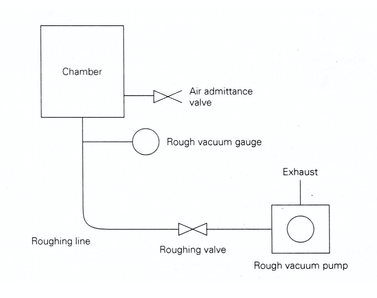
Two other features are needed to complete the rough vacuum system. First, there must be a way of measuring the chamber pressure. This is accomplished by connecting a rough vacuum gauge to the chamber or to the roughing line. The rough vacuum gauge measures the chamber pressure and displays the pressure reading.
Second, there must be a way of returning the chamber to atmospheric pressure from a lower operating pressure so that the chamber can be opened and its interior space accessed. To provide this capability, a vent (air admittance) valve is connected directly to the chamber. When the vent valve is opened, room air at atmospheric pressure (or often dry nitrogen) flows into the chamber and the chamber returns to room pressure.
4.3 Gas Load in the Rough Vacuum Regime
An important concept when working with vacuum systems is gas load. We will define gas load as the amount of gas that has to be removed from the chamber. Contributors, or sources of gas load, vary as the pressure varies and different contributors to gas load do not all equally contribute to the total gas load. Contributors to the gas load will also depend on the types of materials used in the vacuum system design and how the vacuum system is constructed and assembled.
The major contributors to gas load in the rough vacuum regime are the bulk gas, desorption of gas from surfaces, and virtual and real leaks (see Figure 4.2). For the time being, we will assume that there are no real leaks in the system. We will also assume that the system was built without creating sources of virtual leaks. That leaves the bulk gas and desorption of surface gas, mainly water in most cases, as the major contributors to gas load. Other gas load sources, namely bulk outgassing, diffusion, permeation, and backstreaming, contribute negligible amounts in the rough regime, so we will not address them in this chapter.
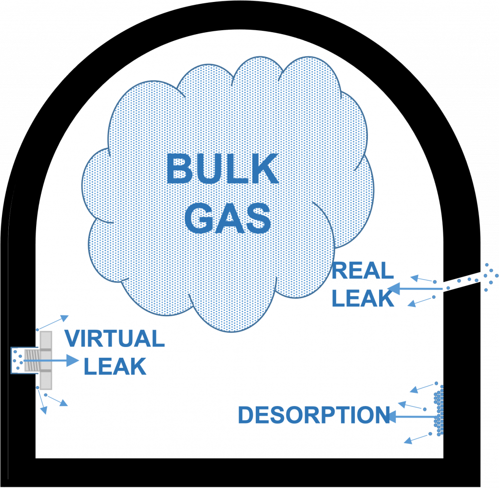
Figure provided by Nancy Louwagie, Normandale Community College.
The bulk gas can be determined by multiplying the chamber pressure by the volume of the chamber plus any other volumes interconnected and open to the chamber. The amount of gas is measured in torr-liters, or an alternative volume-pressure product. For example, a 5-liter chamber at atmospheric pressure (760 Torr) has a bulk gas contribution to gas load of 5-liters multiplied by 760 Torr, or 3,800 Torr-liters of gas. In Chapter 3, Example 3.1 shows how to calculate a volume and use the local atmospheric pressure condition to determine the gas load due to the bulk gas present.
The contribution of surface gas to gas load is harder to quantify. This contribution depends on the surface area, the humidity of the air allowed into the chamber, and the length of time the chamber is exposed to the atmosphere. We may have little control over these variables. Nevertheless, if the system has been vented to the atmosphere, water vapor from the air has coated the inner surface of the chamber, piping, and other system components. As the chamber is pumped down, the water on the inner surface of the chamber will begin to desorb from the surface and enter the gas phase. The bonds between water molecules in the layers nearest the chamber’s surface can take a very long to break. Heating, or baking, the chamber speeds up desorption of water from the inner surfaces of the chamber. Once in the gas phase, those water molecules can be pumped out of the chamber.
4.4 Rough Vacuum Pumps
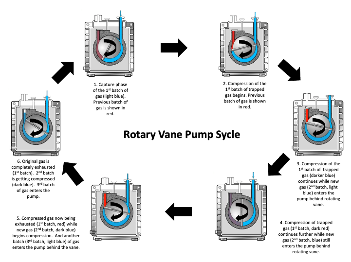
Rough vacuum pumps are called positive displacement vacuum pumps. The operation of a positive displacement pump is based on Boyle’s law applied over many repetitive cycles. Positive displacement pumps repeatedly expand the volume, isolate it, compress the trapped gas, and then expel the trapped gas as shown in the Figure 4.3.

Diagram provided by Nancy Louwagie, Normandale Community College.
To illustrate this process, consider the system shown in Figure 4.4. A piston-type pump is connected to a 10-liter chamber. A pressure gauge and a vent valve are attached to the chamber. The volume within the piston pump is 1-liter. What will the chamber pressure be after five strokes of the piston pump?

Solution:
Initially, the chamber pressure is nominally at 1 atm, or 760 Torr. The piston pump is pushed in so that the interior volume of the pump is zero. The pressure gauge displays a pressure reading of 760 Torr.
We will apply Boyle’s law to determine what happens to the chamber pressure, one stroke of the piston pump at a time.
Stroke 1. When the piston and handle of the pump is drawn back, the pump’s exhaust valve is closed, and the inlet valve of the pump is opened allowing gas from the chamber to flow into the pump. This essentially expands the chamber volume to 11 liters (10-liters in the chamber plus 1-liter in the pump). By applying Boyle’s law, we calculate the pressure in the chamber according to:
Where,
Hence,
When the piston is pushed forward, the pump’s inlet valve closes, and the pump’s outlet valve opens. The gas within the pump is compressed and expelled to atmosphere. When the handle returns to its original position, the volume within the pump is again zero. The first stroke cycle is complete, and fewer gas molecules remain in the chamber volume.
Stroke 2. When the piston is drawn back out again, the outlet valve closes, and the inlet valve opens so the system volume again expands by an additional 1-liter to a total volume of 11-liters. The gas flows from the chamber into the pump volume and the pressure decreases. Again, we apply Boyle’s law to determine the new pressure level using P (after 1 stroke) as the initial pressure. The P (after 2 strokes) is calculated by:
As before, the liter of gas in the pump is isolated. Then, as the piston is returned to its original position, the trapped gas in the pump is compressed and exhausted from the pump. The second stroke cycle is complete, and even fewer gas molecules remain in the chamber.
Stroke 3. When the piston is drawn back a third time, the gas volume again expands to 11-liters. The new pressure is:
Again, the gas cycle (isolation, compression, and exhaust) is repeated. The third stroke cycle is complete.
Stroke 4. When the piston is drawn back a fourth time, the gas volume again expands to 11-liters. The new pressure is:
The fourth stroke cycle is complete.
Stroke 5. Again, the piston is drawn back a fifth time, expanding the gas volume. The new pressure is:
And finally, the liter of gas in the pump is again isolated, compressed, and exhausted. The fifth stroke cycle is complete. Hence, the pressure in the chamber after five strokes of the piston pump is approximately 472 Torr. See the animation below that takes you through this process step-by-step.
Animation 4.1. Piston Pump Example. Animation provided by Elena Brewer, SUNY Erie Community College.
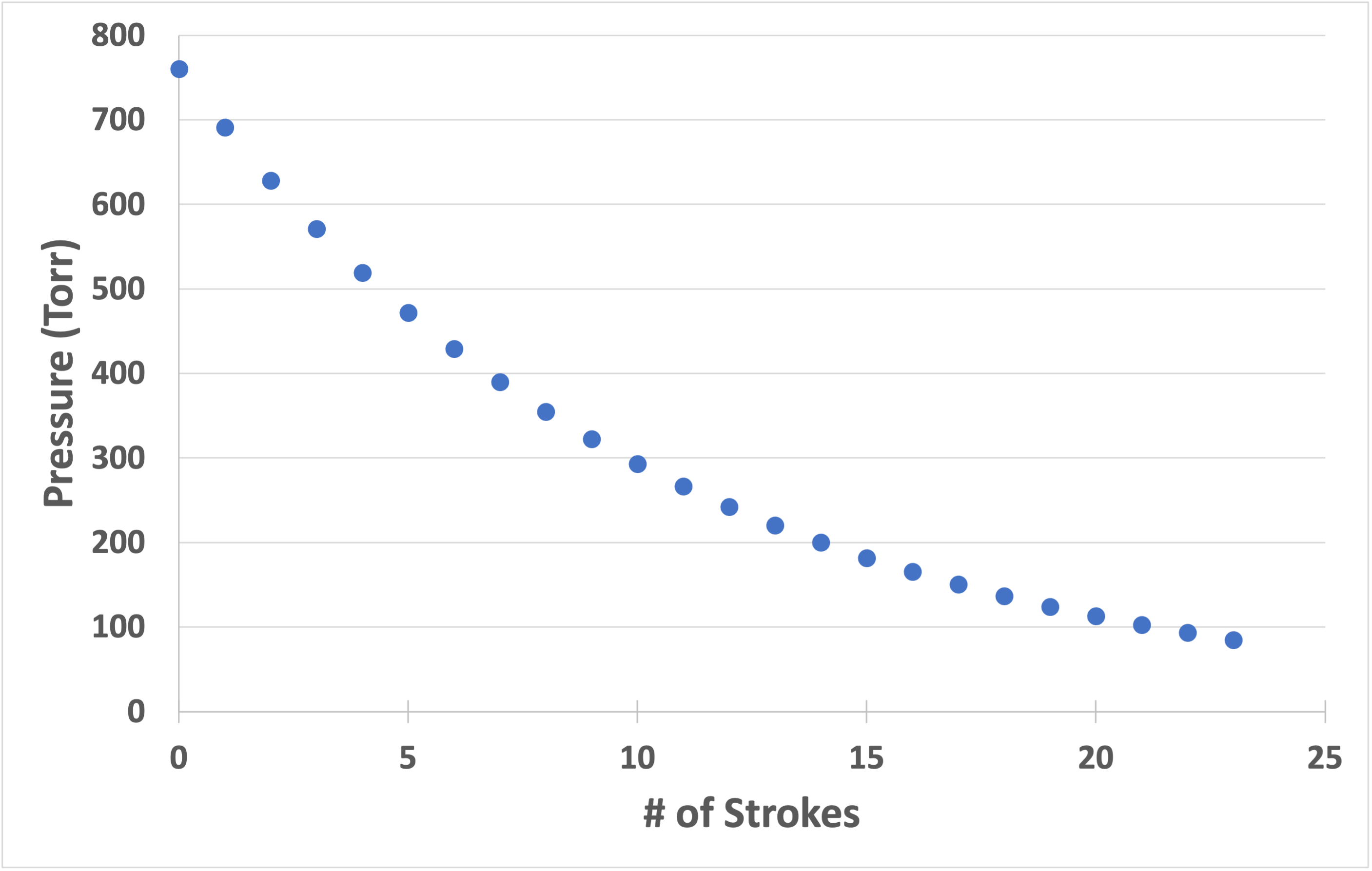
If this example is continued for twenty strokes and a pressure versus strokes graph is plotted, a graph as shown in Figure 4.5 would be obtained. The graph shows an exponential decrease in pressure. This graph is called a pump-down curve. The curve shown in Figure 4.5 asymptotically approaches zero pressure as the number of strokes increases. In practice, it is not possible to achieve absolute zero pressure. The positive displacement pump has a pressure limit below which the Boyle’s law model does not apply due to change in the gas flow characteristics. The actual lowest pressure achieved by a positive displacement pump is called its ultimate pressure.
All positive displacement vacuum pumps use this expansion, isolation, compression, and exhaust cycle to move gas from the pump’s inlet to the pump’s outlet. Let us examine the pumping action of four types of rough vacuum pumps: diaphragm pumps, scroll pumps, rotary vane pumps, and Roots pumps.
4.4.1 Diaphragm Pumps
Diaphragm pumps are one of the basic types of positive displacement pumps. They are simple in design, reliable and relatively low-cost.
When we breathe, our lungs behave like a diaphragm pump. As the diaphragm at the bottom of the chest cavity is pulled down, expanding the volume of the chest cavity, air flows into our lungs. When the diaphragm is pushed up, the volume of the chest cavity decreases, the air in our lungs is compressed, and we exhale. We repeat this pumping cycle over and over again throughout our life.
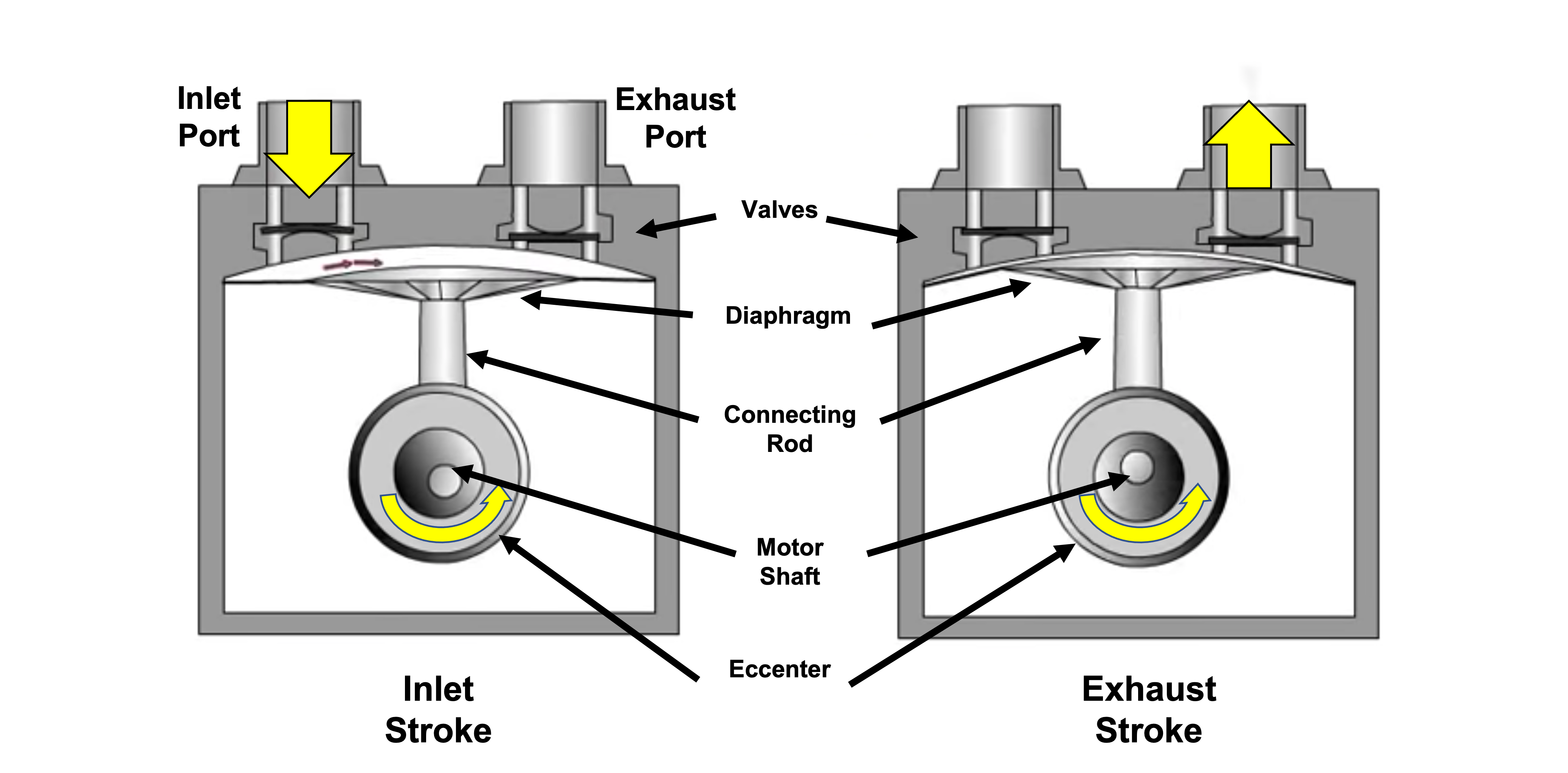
Figure 4.6 shows the pumping mechanism for a diaphragm pump and the corresponding flow of gas through the pump. A diaphragm made of a flexible material forms one wall of a small chamber. The flexible diaphragm is attached to a piston, which is attached to an eccentric cam driven by an electric motor. As the cam rotates, the piston rod moves up and down which acts to push and pull on the flexible diaphragm. When the diaphragm is pulled down, the volume within the pump’s small chamber increases. When the diaphragm is pushed upward, this volume decreases. Animation 4.2 shows the flow of gas through the pump during each pumping cycle.
Animation 4.2. Diaphragm Pump Example. Animation provided by MATEC.
The pumping cycle consists of two phases. During the gas capture phase of operation, the cam rotates, and the piston rod is pulled down. The piston pulls on the diaphragm, the diaphragm stretches which causes the volume within the pump chamber to increase. As the volume within the pump increases, the corresponding pressure in that space decreases. This causes the inlet valve to open, and gas from the chamber flows through the inlet port and into this expanded space within the pump. The second phase begins when the rotation of the cam causes the piston rod to change direction and begin moving upward. This upward motion of the piston pushes the diaphragm up and reduces the volume of the small chamber. The trapped gas gets compressed, and the pressure in the small chamber increases. This causes the inlet valve to close and the exhaust port to open, and the gas is expelled from the chamber. This completes one pumping cycle.
A single stage diaphragm pump is capable of reducing the pressure level to approximately 50 Torr. The lowest pressure a vacuum pump can achieve is defined as its ultimate pressure. Diaphragm pumps may be made with multiple chambers to improve pumping performance. Up to four chambers can be combined in a single pump. A four-stage pump can achieve an ultimate pump pressure of approximately 0.5 Torr. Pumping speeds range from 10 to 60 liters per minute. Most diaphragm pumps operate at either 120 V / 60 Hz or 220 V / 50 Hz.
Diaphragm pumps are best suited for applications that do not require removal of large volumes of gas. One significant functional advantage to using diaphragm pumps is that they are a type of dry pump. A dry pump does not use oil to create airtight seals during operation. Use of dry pumps eliminates back streaming of oil vapor as a gas load source in a vacuum system. Diaphragm pumps are commonly utilized in small analytical systems or as the backing pump for a turbo pump. These systems are used in clean operating environments. Another important consideration in vacuum pump selection is the cost of the pump. Diaphragm pumps tend to be relatively inexpensive compared to other positive displacement pumps. Diaphragm pumps are also attractive because they are ambient air-cooled, rather than water-cooled.
Maintenance tasks associated with a diaphragm pump are easy to perform. The diaphragm should be replaced routinely to maintain optimal pump performance. Generally, the replacement period for a diaphragm is after every 10,000 hours of operation. Replacing the diaphragm is not difficult. Sub-components associated with the pump’s inlet and outlet valves, like gaskets, may also need to be replaced. If the diaphragm pump starts exhibiting an increase in its ultimate pressure, the condition of the diaphragm and possibly the valve components should be checked and/or replaced.
Drawbacks to using diaphragm pumps are their inherently low pumping speed and high ultimate pressure. Because of these two limitations, diaphragm pumps are not used as the primary roughing pump in large-scale manufacturing applications.
Diaphragm Pump Key Takeaways:
|
Diaphragm Pump Advantages |
Diaphragm Pump Limitations |
|
|
4.4.2 Scroll Pumps
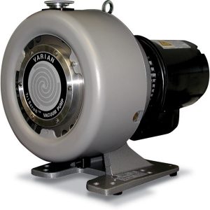
Another type of positive displacement pump is a scroll pump. The scroll pump, like the diaphragm pump, is a type of dry pump. Oil-free scroll pumps like the one shown in Figure 4.7 provide clean operating environments with no sealant or lubricant required in the vacuum-exposed region. They are ambient air-cooled and do not require cooling water. Scroll pumps are capable of much higher pumping speeds than diaphragm pumps and can achieve a lower ultimate pressure. Scroll pumps are used extensively in systems that support manufacturing processes conducted in very clean environments like semiconductor manufacturing.
Scroll pumps use two scrolls, or plates, shaped into a spiral called an involute curve. The two scrolls fit inside one another. The edge of the scroll is covered by a tip seal. One scroll is fixed in place and remains stationary during operation. The other scroll moves with an orbital motion around the stationary scroll. The scroll pump design does not include an inlet valve component like the diaphragm pump design. Instead, the orbiting motion of the movable scroll continually traps pockets of gas and compresses each pocket to the point at which the gas is expelled from the pump.
The motion of the scroll pump creates a crescent shaped volume that repeatedly opens to the vacuum system and serves to expand the system volume. The pressure in the vacuum chamber decreases as the gas flows out of the chamber through the system and into the pump. After gas flows into the crescent shaped pocket, the one scroll plate continues its orbital motion, and the gas pocket seals (see Figure 4.8 and Animation 4.3). The crescent shaped pocket shrinks as the movable scroll continues in its orbital trajectory, and the trapped gas is compressed. The trapped gas moves along the scroll toward the center of the scroll. When the pocket of gas reaches the center, it is expelled through the pump’s outlet. The sequence of gas capture, gas compression, and gas exhaust is performed over and over again as the movable scroll moves in this orbital trajectory.

Animation 4.3. Dry Scroll Pump Mechanism Animation. Animation provided by MATEC.
Scroll pumps offer several functional advantages. Scroll pumps are dry, have high pumping speeds, and achieve low ultimate pressures. Using a scroll pump eliminates the risk of oil contamination and the need for oil traps and eliminators. Pumping speeds range from 300 to 600 liters per minute. Scroll pumps can reach ultimate pressures from 0.01 (10-2) Torr to 0.001 (10-3) Torr. Scroll pumps can also be configured for either single-phase or three-phase operation at 50 Hz or 60 Hz.
Routine maintenance tasks associated with a scroll pump are relatively easy to perform. The tip seal should be replaced regularly to maintain optimal pump performance. Service intervals are specified by the vendor and often are around 10,000 hours of continuous operation. The process of replacing the tip seal is not difficult. If the scroll pump starts exhibiting an increase in its ultimate pressure during operation, the tip seal should be replaced. The tip seal should also be replaced if the pump emits excessive particulate during operation. However, if a scroll pump is emitting excessive amounts of particulate, this may be an indication that a scroll pump is not suitable for the process being run or there is a problem with the underlying process.
Scroll pumps are intended for use in clean environments to support clean, dry processes. Any particulate or liquid state matter present in the gas load can damage the scroll pump. A gas ballast may be included on a scroll pump to help prevent certain vapors from condensing as they are compressed by the pump. The ballast function will be explained in more detail in the section addressing the rotary vane pump. A drawback to scroll pumps is that the pump itself can be the source of particle generation as the tip seal wears out. Scroll pumps as an initial investment are also moderately expensive compared to some other rough pump types.
Scroll Pump Key Takeaways:
|
Scroll Pump Advantages |
Scroll Pump Limitations |
|
|
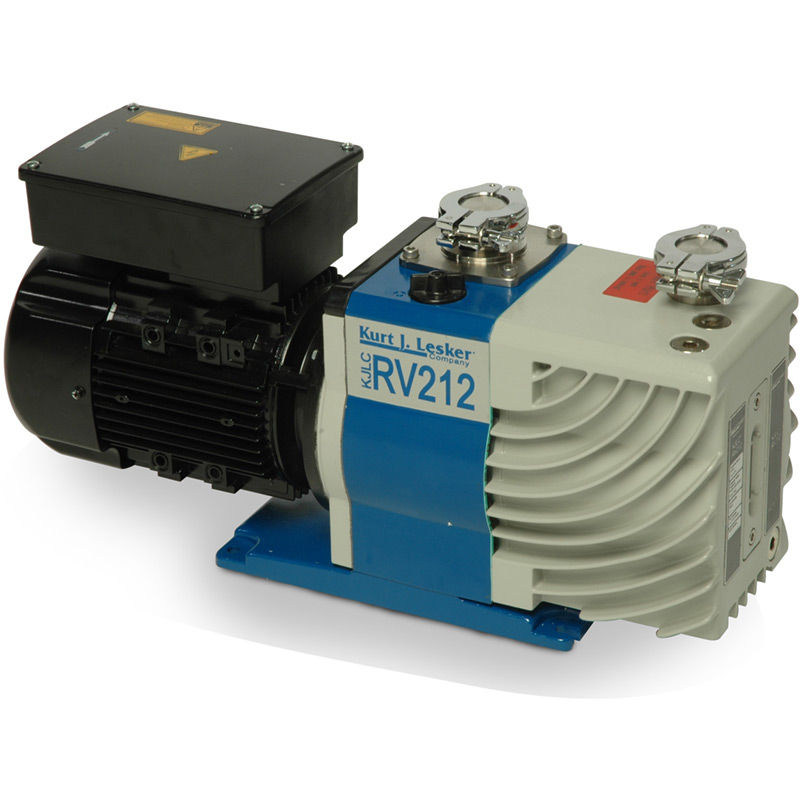
4.4.3 Rotary Vane Pumps
One of the very first mechanical vacuum pumps was a piston type as described in Section 4.4. A successor to the piston pump was a mechanical, mercury-sealed rotary pump. Today the rotary vane pump is one of the most commonly used vacuum pumps. A rotary vane pump is shown in Figure 4.9. The rotary vane pump works on the same principle as the diaphragm pump and the scroll pump. As the pump cycles, volumes of gas are repeatedly expanded, trapped, and expelled. The pressure in a chamber connected to the pump decreases over successive cycles of pump operation. Unlike the diaphragm pump and scroll pump, the function of the rotary vane pump requires the use of oil. The oil serves important functions in rotary vane pump operation. First, oil lubricates moving parts in the pump to reduce frictional wear. Second, the oil equilibrates and dissipates heat generated during the pump’s operation. And finally, the oil makes a seal which traps each volume of gas that is subsequently compressed and expelled.
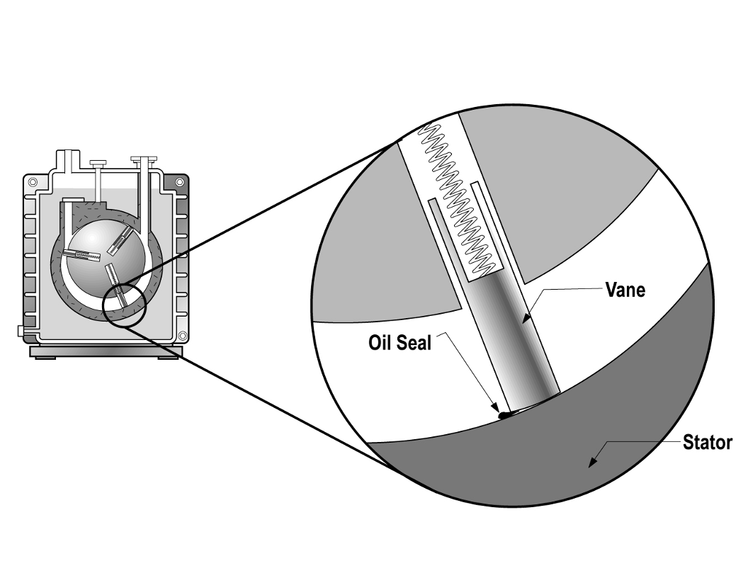
The pumping mechanism in a rotary vane pump is enclosed by a stator as shown in Figure 4.10 (a). Inside the stator is an offset rotor that is mechanically coupled to a drive motor. The drive motor turns the offset rotor that contains spring-loaded vanes. A small amount of oil in Figure 4.10 (b) forms the seal between the end of the sliding vanes and the inner surface of the stator. As the rotor turns, a sealed space within the pump is created.
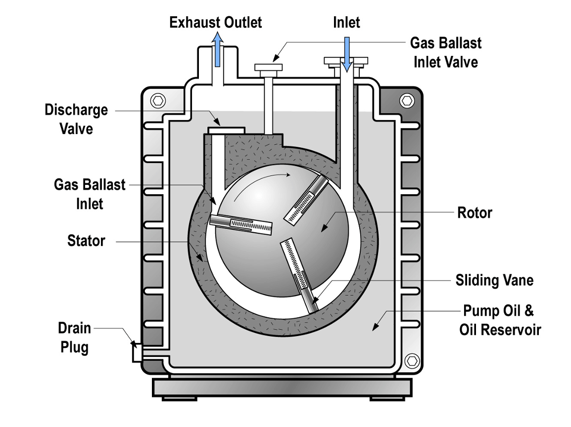
Let’s examine the operation of a rotary vane pump in more detail. Again, a cross-sectional view of a rotary vane pump is shown in Figure 4.10(a). As the sliding vane passes by the opening to the inlet port, gas molecules begin to flow into the space behind the sliding vane. As the space behind the sliding vane increases, more gas molecules flow into this space. Eventually, the other end of the vane passes the inlet opening and seals off the volume of gas molecules that have moved into the pump.
As the rotor continues to rotate, the trapped volume of gas is gradually compressed and the pressure of the trapped gas increases. The compressed gas is then opened to the exhaust port. If the pressure of the trapped gas is greater than the pressure on the other side of the discharge valve, the discharge valve opens, the trapped gas escapes into the exhaust line and exits through the exhaust port. This process repeats twice for each rotation of the sliding vane if a two-vane pump is used as shown in Figure 4.10 (c). However, if the pressure of the trapped gas is insufficient to open the gas discharge valve, then the gas stays in the pump and no gas is exhausted from the pump. Figure 4.10(c) shows snapshots in time illustrating the movement of gas through the pump.
If the discharge valve does not open, there is a risk of vapor condensation and contamination of the pump oil. If the oil becomes contaminated with water or other impurities, these contaminants will increase the vapor pressure and make it impossible, or at least more difficult, to reach satisfactory base pressures.
A gas ballast feature is often used to ensure that the discharge valve opens during every cycle. The ballast valve opens during each cycle, allowing a quantity of air, or an inert gas, to be admitted during the compression cycle. This extra gas ensures that the pressure of the compressed gas is great enough to open the discharge valve, allowing condensable vapors to exit the pump before they condense inside the pump. Without the extra gas admitted through the gas ballast mechanism, some of the vapors present will condense inside the pump if the gas reaches its saturation vapor pressure during the compression phase. The downside of the ballast function is an increase in the ultimate pressure of the pump.
When oil-sealed mechanical pumps are operated at low pressures, they tend to backstream oil vapor back into the roughing line and process chamber. This may affect the process being run. Oil migration can be controlled by inserting traps, such as molecular sieve traps, in the roughing line. Another solution is to use oil-free mechanical pumps, such as diaphragm pumps and scroll pumps.
Rotary vane pumps are very popular pumps and used in many applications. This type of rough vacuum pump offers several functional advantages. Rotary vane pumps can achieve high pumping speeds and low ultimate pressures, are relatively easy to use, and if maintained properly, are rugged and durable. These pumps come in a variety of sizes and support different levels of pumping capabilities. They also come in a wide range of pumping speeds spanning from approximately 10 liters per minute up to 20,000 liters per minute. Rotary vane pumps can reach ultimate pressures as low as 0.001 (10-3) Torr without a ballast. When the gas ballast is used, a rotary vane pump’s ultimate pressure increases by approximately a factor of 10. Rotary vane pumps are available as one-stage or two-stage pumps. Some two-stage pumps are capable of higher pumping speeds and lower ultimate pressures than one-stage pumps. These pumps can be selected for either 120 VAC / 60 Hz or 220 VAC / 50 Hz operation.
It is important to maintain a rotary vane pump properly to ensure its optimum performance. Maintenance tasks associated with a rotary vane pump are relatively easy to perform. The pump’s oil should be inspected routinely and changed regularly. It is important to use the right type of oil with this pump. The oil used with a rotary vane pump should have a low vapor pressure, for example, as low as 0.075 milliTorr at room temperature. If the oil looks like it is chemically reacting (often with water) such that it is acquiring a milky green appearance, it should be changed immediately. Other mechanical parts and accessories like the springs, blades, rotor, stator, valves, seals, filters, and traps on the pump can be replaced if they malfunction or wear out.
Rotary vane pumps are versatile and used in a variety of manufacturing environments. These pumps, when maintained properly, provide dependable performance for a long time. The major drawback to rotary vane pumps is the presence of the oil which can vaporize and cause problems for certain processes. Rotary vane pumps are typically the least expensive of the rough pump options, but the price of this pump can vary greatly. The low vapor pressure oil used with these pumps can be expensive. This represents an on-going operating expense that needs to be considered when selecting this type of pump.
Rotary Vane Pump Key Takeaways:
|
Rotary Vane Pump Advantages |
Rotary Vane Pump Limitations |
|
|
4.4.4 Roots Vacuum Pumps
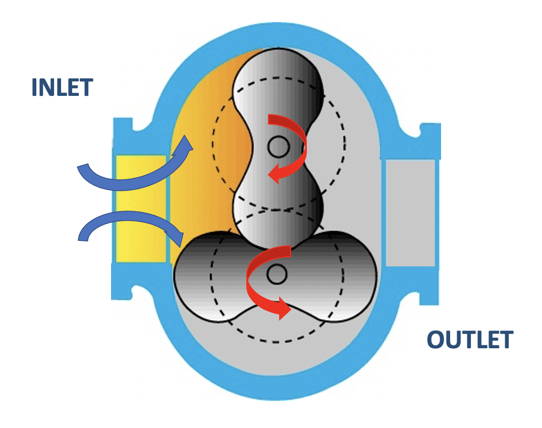
One rough vacuum pump that operates differently from the pumps previously described is the mechanical booster pump. This positive displacement pump is better known as a lobe blower or the Roots pump. Like previous rough pumps, a volume within the Roots pump expands allowing gas molecules from the chamber to move into the pump, the pump’s motion traps the gas molecules and transfers the gas to the pump’s exhaust. The Roots pump differs from the previous pumps because this pump does not include valves at its inlet and outlet. The Roots pump functions to transport gas molecules from the inlet to the outlet very rapidly.
The Roots pump accomplishes the pumping function through the rotation of a meshed lobed rotor mechanism with impellers mounted on parallel shafts and rotating in opposite directions. Figure 4.11 shows a cross-section of a mechanical booster pump with two-lobe rotors. The arrows show the direction of rotation by the rotors and the resulting flow of the gas molecules within the pump. The rotors do not touch each other as they rotate, nor do they make contact with the surrounding walls (stator). The clearances between the rotor faces and other surfaces are generally less than 0.5 mm. The rotors spin at speeds between 1,400 and 4,000 revolutions per minute. The high rotational speeds are possible because the speed of the lobes is not reduced by friction with the stator.
The Roots pump is frequently operated in combination with another type of positive displacement pump. Since the rotor faces within a Roots pump do not completely seal during their pumping motion, gas molecules from a single-stage Roots blower can easily leak from the pump outlet back toward the chamber. The result is that a Roots pump operating by itself achieves a very low pumping speed when it exhausts the trapped gas to atmosphere.
A Roots pump rapidly passes the gas through the pump without compressing the gas appreciably. Therefore, a single Roots pump cannot exhaust directly to atmosphere. The outlet of a Roots pump is connected to the inlet of another positive displacement pump which serves as a backing pump. The backing pump compresses and exhausts the gases to atmosphere. In some systems, the Roots pump is not energized as the system starts pumping down from atmosphere. Instead, the backing pump does the initial work to start the pump-down process from atmosphere. During the initial stage of the pump-down process, the Roots pump impellers rotate freely allowing gas to flow through the Roots pump. When the inlet pressure to the backing pump reaches a pressure of approximately one to ten Torr, the Roots pump is energized so the impellers become actively driven. After this point in the system pump-down process, the Roots pump will increasingly function to enhance the pumping speed of the system as the system continues to pump down through the pressure range of one Torr to 1×10⁻³ Torr.
The Roots pump is susceptible to generating high levels of heat. As stated previously, the Roots pump design does not function to support high compression ratios. Attempting to operate the Roots pump starting at atmosphere can overload the pump motor and cause the pump to overheat. The backwards movement of molecules through the Roots pump, especially smaller molecules like hydrogen and helium, compounds the heat generation problem.
Making a few careful considerations in the design and operation of a vacuum system with a Roots pump will help to avoid excessive heat generation by the Roots pump. It is important to pair a Roots pump with an appropriate backing pump. The pumping speed of the Roots pump should be limited to no more than a factor of two to eight times greater than the pumping speed of the backing pump. During its operation, the pressure difference between the outlet of the Roots pump and its inlet should not exceed the manufacturer-specified limit. Some Roots pumps are designed with a bypass line and relief valve that help to limit the pressure difference between the outlet and the inlet of the pump. Other Roots pump models include gas coolers in their design that allow the pump to tolerate larger pressure differences between the outlet and the inlet during operation. And some Roots pump models automatically slow down at high pressures to avoid generating excessive heat or overloading the motor.
Since Roots pumps are effective at pumping on large volumes and achieving low system base pressures, they are used in a variety of manufacturing and research environments. Roots pumps in combination with an appropriate backing pump achieve the highest pumping speeds through the medium vacuum range at up to 50,000 liters per minute. Vacuum systems with a Roots pump can achieve ultimate pressures below one milliTorr. Compared to other positive displacement pumps, the Roots pump is typically more expensive due to the complexity of the pump design. Multi-stage Roots pumps models are also available. Like the other positive displacement type pumps, Roots pumps can be selected for either 120 VAC / 60 Hz or 220 VAC / 50 Hz operation.
When properly operated and maintained, these pumps are very durable and provide dependable performance for long periods of time. The Roots pump, like the diaphragm and scroll pump, is a type of dry pump that can help limit backstreaming from an oil-sealed rotary vane pump. Although oil is used to lubricate the gears and bearings in a Roots pump, no oil is present in the gas flow space. It is important to maintain an oil fill level in the pump that properly lubricates the inner gear teeth that drive the impellers. Lubricants and oils should provide the right level of viscosity over the range of pump operating temperature.
Roots Pump Key Takeaways:
|
Roots Pump Advantages |
Roots Pump Limitations |
|---|---|
|
|
4.4.5 Other Rough Vacuum Pumps
There are other types of commonly used rough vacuum pumps. These pumps include rotary piston pumps, claw pumps, and screw pumps. Each pump implements the gas capture, compression, and gas exhaust cycles using different geometries. A very brief description for each of these pumps is provided in this section. See the references for additional information about the design and operation of each of these pumps.
Rotary piston pumps are similar to rotary vane pumps. The eccentric cam drives a piston that draws a volume of gas into the pump, isolates the volume, compresses it, and exhausts it. Pumps of this kind are typically used as roughing pumps on large vacuum systems either alone or in combination with a Roots pump. They are rugged and mechanically simple, providing high pumping speeds.
Claw pumps use two claws rotating in opposite directions, like the Roots pump, to capture, compress, and exhaust the gas. Claw pumps can be used to effectively pump corrosive and abrasive gases. They are often combined with Roots pumps to achieve high pumping speeds and pressures in the millitorr range.
Screw pumps are also used to pump corrosive and abrasive gases. These pumps find application in backing turbomolecular pumps in reactive-ion etching and chemical vapor deposition systems. The screw pump uses a pair of large rotating screws to move the gas from the inlet end of the pump to the exhaust end. Like claw pumps, screw pumps have high pumping speeds and ultimate pressures in the millitorr range.
Table 4.1 summarizes vacuum pumps that were discussed in Section 4.5 and compares their main characteristics: pumping speed, ultimate pressure, backstreaming oil, reliability, noise/vibration level, ability to handle corrosive/abrasive gases and condensable gases/vapors, and cost.
Table 4.1. Rough vacuum pumps summary.
|
Characteristics: |
Diaphragm Pump |
Scroll Pump |
Rotary Vane Pump |
Roots Pump |
|---|---|---|---|---|
|
Typical Pumping Speeds (liters/min) |
12 – 167 |
300 – 600 |
17 – 16,000+ |
Up to 50,000 |
|
Typical Ultimate Pressure (Torr) |
1 -38 |
10-2 – 10-3 |
10-1 – 10-3 |
10-2 – 10-4 |
|
Dry vs Wet |
Dry |
Dry |
Wet |
Dry |
|
Oil Backstreaming |
No |
No |
Yes |
Possible –
|
|
Typical Noise Level (dB(A)) |
50 – 55 |
47 – 65 |
48 – 80 |
Various |
|
Can be used to pump abrasive and corrosive gases |
|
Somewhat – |
Somewhat – |
Somewhat – |
|
Can be used to pump condensable gases/vapors |
No |
No |
No |
No |
|
Cost |
Low |
High |
Low |
High |
4.5 Rough Vacuum Gauges
The vacuum pump functions to create the lower pressure condition within a system and specifically within the vacuum chamber. A vacuum gauge measures the level of vacuum present in the vacuum chamber and at other points in the system. Measurements of pressure help us understand and respond to a vacuum system’s performance. There are different types of vacuum gauges available to measure pressure. Each type of gauge has certain features that are useful in a working vacuum system. Each gauge also presents with some limitations for its use. It is important to understand how the different types of gauges function in order to appropriately utilize the measurement data they generate.
As we discussed in Chapter 3, vacuum gauges are classified as either direct reading or indirect reading. Direct reading vacuum gauges measure pressure in the rough vacuum regime. This gauge type measures pressure based on the force exerted by the gas on an area. At pressures between atmosphere down to 1×10⁻³ Torr, the molecular density of the gas is high enough to exert forces that can be detected mechanically. On the other hand, indirect reading vacuum gauges infer the pressure based on measuring another property of the gas that changes predictably as the gas density changes. Vacuum gauges that measure pressure based on heat transfer principles also provide a reliable indication of rough vacuum pressures. At pressures below 1×10⁻⁴ Torr, other indirect measurement techniques are required.
How well will the vacuum gauge measure the pressure in the chamber? This question is a very important one to consider. All measurement devices are inaccurate to some extent. The accuracy of a measurement device is determined by the device’s capability to display a reading that falls within a band defined as an upper limit and lower limit of what is thought to be the true value. The closer the upper limit and lower limit values are to one another, the more accurate the measurement. Vacuum gauges can often be calibrated by the manufacturer or the user to improve their accuracy.
The following sections will describe the behavior of four types of rough vacuum gauge technologies: Bourdon, capacitance diaphragm, thermocouple, and Pirani gauges. There are also measurement devices that combine two different gauge type technologies, like the capacitance diaphragm and Pirani, into a single package. This kind of vacuum gauge is called a combination gauge.
4.5.1 Bourdon Gauges
A Bourdon pressure gauge was patented by Eugene Bourdon in France in 1849. Two years later, Bernard Schaeffer patented a successful diaphragm pressure gauge. Together, the two pressure gauges revolutionized pressure measurement in industry. They were widely adopted for their superior sensitivity, linearity, and accuracy at that time. These low-cost gauges are still used today to measure pressure levels above 1 Torr.
A commercially-available Bourdon pressure gauge is shown in Figure 4.12. This is a direct reading gauge. It operates on the principle that a curved, flattened tube often of non-circular cross-section will straighten when pressure inside the tube increases or will curl when the pressure decreases. To magnify the effect of the pressure change, the tube is formed into a C-shape, or even a helix, so that the entire tube tends to straighten out or uncoil elastically as it is pressurized and will coil when the pressure decreases.
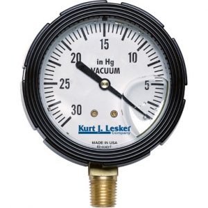
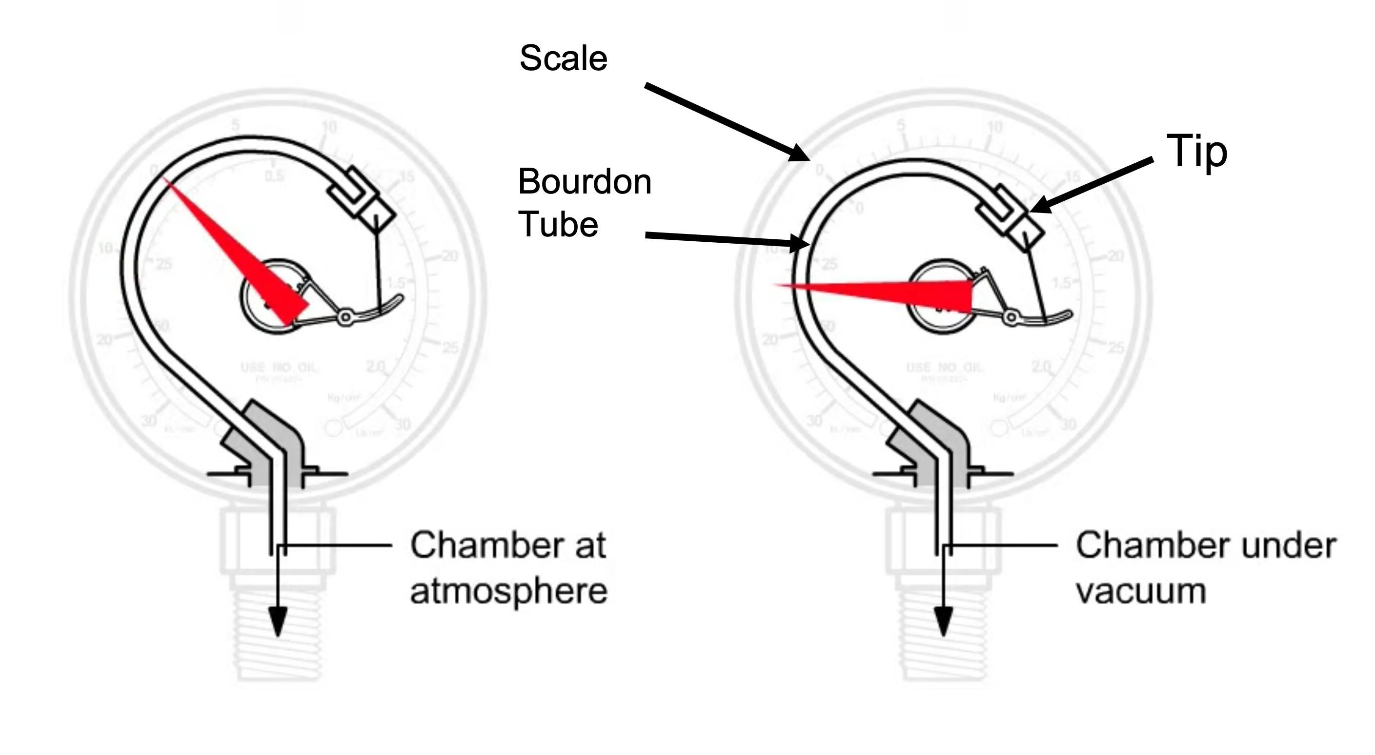
Figure 4.13 shows the internal structure of a Bourdon pressure gauge. The C-shaped Bourdon tube is open at one end and sealed at the other end. As the tube responds to changes in pressure, the movement of the tip is transmitted mechanically through an adjustable link to a segmented lever. The segmented lever rotates around a pivot point and the sector gear end meshes with a pinion gear. As the pinion gear rotates, it moves the attached needle. As the needle moves over the scale, the needle tip indicates the pressure reading. Animation 4.9 demonstrated operation of a Bourdon pressure gauge.
Animation 4.9. Bourdon Pressure Gauge Animation. Animation provided by MATEC.
A Bourdon pressure gauge measures pressure relative to ambient atmospheric pressure, as opposed to absolute pressure. A reading of zero on most Bourdon gauges indicates atmospheric pressure. As the pressure detected by the Bourdon gauge decreases to levels less than atmospheric pressure, the internal coil retracts, and the needle moves to indicate a non-zero value.
Gage pressure is related to absolute pressure and atmospheric pressure by the equation,
If a Bourdon gauge displays the pressure in a vacuum chamber as 5.50 in Hg vacuum, what is the approximate absolute pressure within the chamber?
Solution:
If the chamber’s specific location is not provided, assume that Patmospheric is equal to standard atmospheric pressure, that is, 29.92 in Hg for Earth at sea level.
The known values are:
Substituting these values in Equation 4.1 gives,
For the same pressure measurement in the previous example, what is the absolute pressure within the chamber in units of inches of Hg if the system is located in Denver, Colorado?
Solution:
Denver, Colorado is located at an altitude of roughly 1 mile above sea level. The atmospheric pressure decreases as you move to higher altitudes and get farther away from sea level. At sea level the atmospheric pressure is nominally 760 mm Hg, or 760 Torr. Assume that the typical atmospheric pressure in Denver, Colorado is 615 mm Hg.
The known values are:
We use,
In order to solve for Pabsolute in Equation 4.1, the values of Pgage and Patmospheric must be of the same unit of measure, that is, inches of Hg (in Hg).
We will convert the value Patmospheric from units of mm Hg to in Hg:
Substituting the converted Patmospheric value:
The Bourdon gauge in Figure 4.14.a displays a measurement of the pressure within a vacuum chamber. What is the absolute pressure within the chamber in units of mbar?
Figure 4.14.b displays the barometric pressure condition in the room in which the vacuum chamber is located.
-
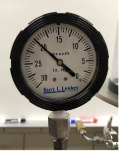
- Figure 4.14.a. Bourdon gauge measurement of pressure inside a vacuum chamber. Photo provided by Nancy Louwagie, Normandale Community College.
-
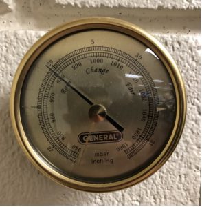
- Figure 4.14.b. Barometric pressure measurement in the room. Photo provided by Nancy Louwagie, Normandale Community College.
Solution:
The known values are:
We use,
In order to solve for Pabsolute in Equation 4.1, the values of Pgage and Patmospheric must be of the same unit of measure, that is, mbar.
We will convert the value Pgage from units of in Hg to mbar:
Substituting the converted Pgage value:
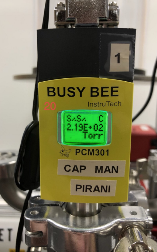
A second gauge measuring the pressure within the vacuum chamber displays the reading shown in Figure 4.14.c when the Bourdon gauge reads 20.00 in Hg vacuum. How do the measurements from the two gauges compare?
Solution:
Since the unit of measure displayed on the gauge in Figure 4.14.c is in torr, we know the measurement displayed by the gauge reflects an absolute pressure.
Convert the value displayed on the gauge in Figure 4.14.c from units of torr to mbar:
The percent difference between the value calculated for the Bourdon gauge measurement and the measurement on the second gauge shown in Figure 4.14.c is:
If the pressure within a vacuum chamber is 488 Torr, what measurement value will a Bourdon gauge display as the pressure in units of in Hg vacuum? The atmospheric pressure is 734 Torr.
Solution:
The known values are:
We use,
This result implies that the measured pressure is 246 Torr less than the prevailing atmospheric pressure.
We will convert the value Pgage from units of torr to in Hg:
The Bourdon gauge is a purely mechanical device. No electrical power is required to operate a Bourdon gauge. Thus, one advantage of using a Bourdon gauge is it will continue to display the pressure condition within a vacuum system if the system loses power. Another advantage of the Bourdon gauge is its fast response time. The disadvantage of a purely mechanical device is that without electronics, a system operator must directly observe and interpret, and, if necessary, hand record the measurement value right at the gauge. Another limitation of the Bourdon gauge is that it does not measure very accurately. A Bourdon gauge provides just a general indication of the vacuum level present. The rate at which the needle moves on the Bourdon gauge provides an idea of how fast a vacuum system is pumping down. When a Bourdon gauge needle stays at zero after a pump down sequence has been initiated, most likely a gross leak is present in the system.
4.5.2 Capacitance Diaphragm Gauges
A capacitance diaphragm gauge, or capacitance manometer, is also a direct reading gauge. It senses the deflection of a flexible metal diaphragm in the gauge produced by the collective force of many gas molecules striking the diaphragm. The metal diaphragm functions as a boundary that separates two spaces. One space is evacuated and permanently sealed. This space provides a vacuum reference pressure. The space on the opposite side of the diaphragm is open to the gases present in the vacuum system. The metal diaphragm forms part of a capacitance circuit. Since,
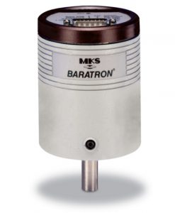
where C is the capacitance in farads, ε is the permittivity of the dielectric material, A is the plate area, and d is the plate separation, capacitance is inversely proportional to the distance between the two plates forming the capacitor. Note, plate area and the dielectric material do not change. The electronic circuitry in the gauge controller converts this change in capacitance to a corresponding frequency and then to a pressure readout. Figure 4.15 shows a capacitance manometer gauge.
Capacitance manometers are used as process-control monitors because they are gas species independent and can be very accurate. They can provide highly accurate measurements over almost seven decades of pressure from 1,000 Torr to approximately 1.0 x 10⁻⁴ Torr. However, it may be necessary to use two or three capacitance manometer gauges if you want to make accurate measurements over this full range of pressures. Capacitance manometers are calibrated to take accurate readings within a smaller range of pressures. The measurement range of any one capacitance manometer is typically limited to two or three decades of pressure, for example from 10 Torr to 1,000 Torr for two decades or 0.01 Torr to 10 Torr for three decades. They are very fast, with response times on the order of 1 millisecond or less and have an accuracy of ± 0.25%, or less, of full scale. The downside of using capacitance manometers is that they are more expensive than other gauges within the same pressure range, such as thermocouple and Pirani gauges.
4.5.3 Thermal Conductivity Gauges
A gas has the ability to carry away heat. Conduction is a form of heat transfer in which individual molecules transfer heat from hotter to colder regions. After an air molecule collides with and rebounds from a heated surface, it carries away some of the surface heat energy. An increase or decrease in the number of air molecules present to collide with a heated surface causes a corresponding increase or decrease in the rate at which heat is carried away from the surface. We are familiar with thermos bottles. As was described in Chapter 1, the thermos bottle design consists of a smaller flask inserted within a larger flask. Air is removed from the sealed space to create a vacuum condition. By reducing the molecular density in the space between the inner flask and the exterior wall of the thermos bottle, the rate of heat transfer to or from the liquid inside the thermos bottle is reduced. In this way, we can keep cold liquids cold and hot liquids hot.
Thermal conductivity gauges are a type of indirect-reading pressure measurement gauge. The term indirect reading implies that the gauge does not measure pressure directly, but instead measures some other parameter associated with the gas and then converts it to a pressure reading. The operating principle employed by a thermal conductivity gauge is based on the ability of a gas to conduct heat. As the name implies, a thermal conductivity gauge measures temperature and then translates or converts the temperature to a pressure reading.
Thermal conductivity gauges operate by measuring how much heat is lost from a heated surface as the molecular density surrounding the surface changes. The heated surface in a thermal conductivity gauge is created by passing electric current through a very thin filament wire. Heat is lost from the surface of the wire every time a gas molecule hits it and rebounds back into the chamber, taking some heat energy from the wire’s surface. Higher pressures mean more collisions between gas molecules and the heated filament surface which results in a high rate of heat loss. Conversely, lower pressures mean fewer collisions between gas molecules and the surface, and consequently a lower rate of heat loss. The amount of heat loss can be measured using either Fahrenheit, Celsius, or Kelvin temperature scales. Thermal conductivity gauges are effective at measuring pressures in the lower range of the rough vacuum regime, that is, pressures between 0.001 and 10 Torr.
4.5.3.1 Thermocouple Gauges
A thermocouple gauge is one type of thermal conductivity vacuum gauge. The function of this gauge is enabled by a thermocouple sensing element. A thermocouple consists of two different metals joined together. The joining of two dissimilar metals produces a small electrical voltage. Heating or cooling the thermocouple causes corresponding changes in the junction voltage. Thus, a thermocouple behaves like an electric thermometer.
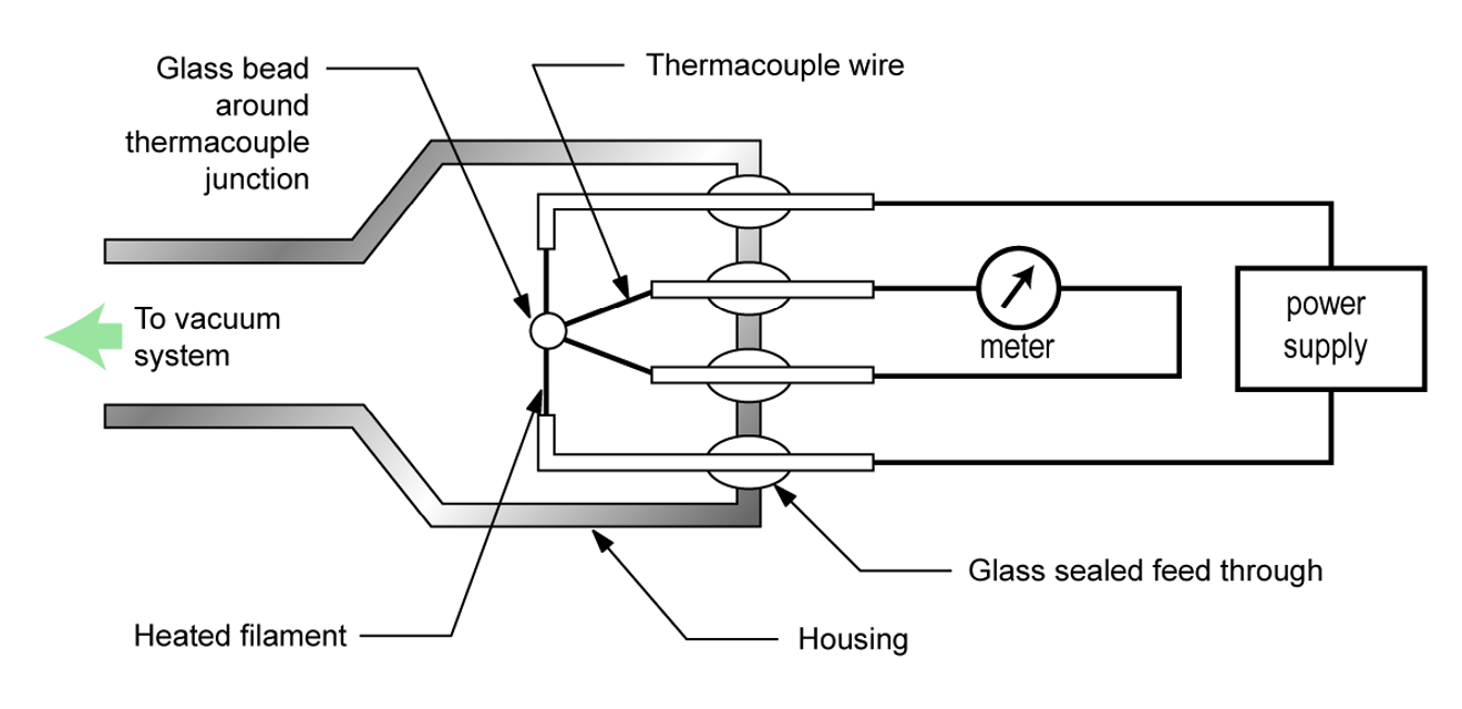
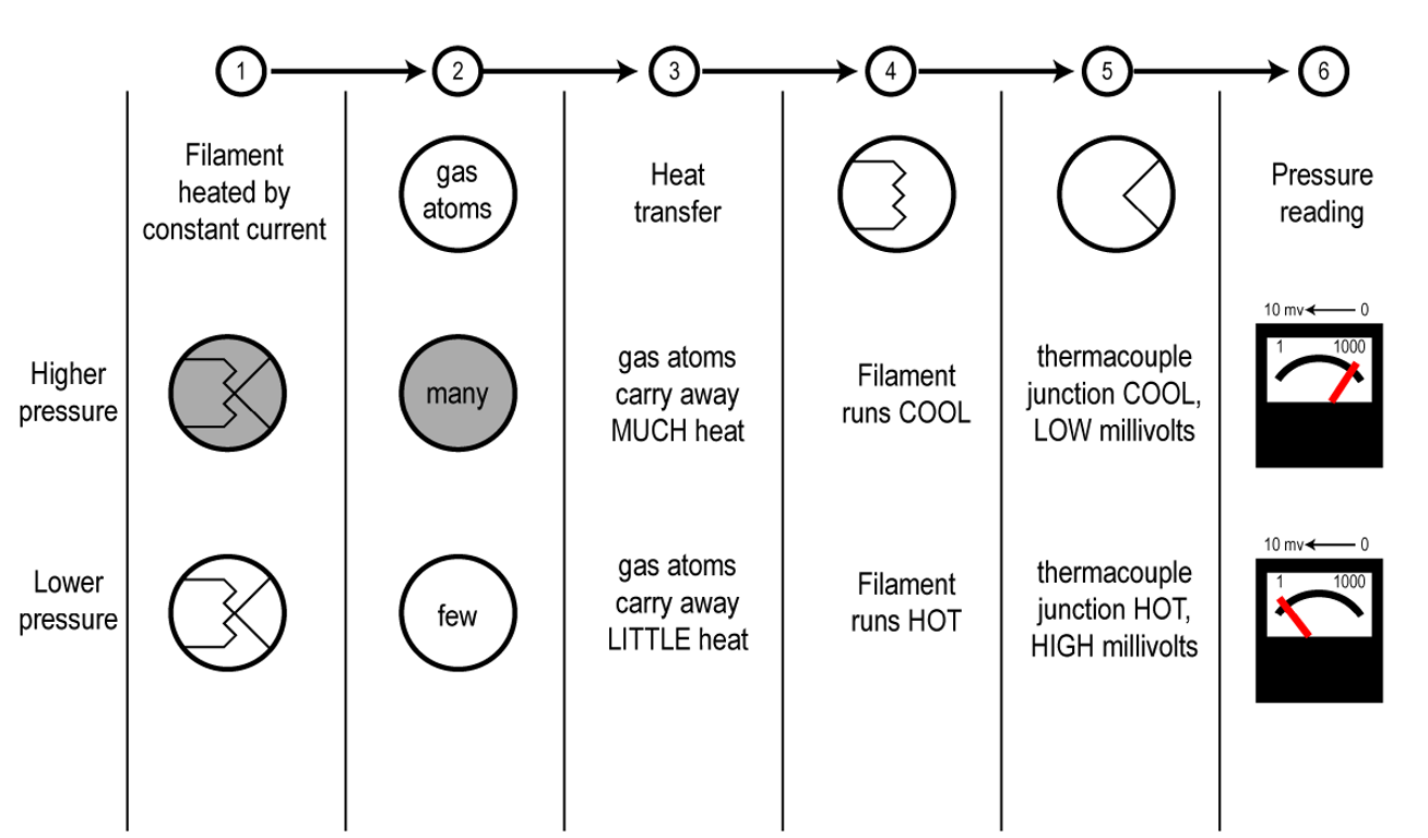
Figure 4.16 (a) shows the construction of a thermocouple gauge. The gauge controller applies a set voltage to the filament to heat it up to its operating temperature. As the pressure decreases around the filament, fewer gas molecules are available to carry away the filament’s heat energy. As a result, the filament gets hotter as shown in Figure 4.16 (b). A thermocouple is attached to the filament to sense the temperature of the filament. The gauge controller monitors the voltage produced by the thermocouple and produces a pressure reading that corresponds to the magnitude of the voltage.
The useful measurement range of a thermocouple gauge is approximately between 0.01 and 1 Torr. Some thermocouple gauge designs include enhancements which expand the measurement range slightly. The measurement accuracy of a properly calibrated thermocouple gauge for a specified gas type is approximately ±15%. Some of these gauges can be calibrated at the lower end of the measurement range by adjusting the temperature of the heating filament. Thermocouple gauges are relatively inexpensive.
4.5.3.2 Pirani Gauges
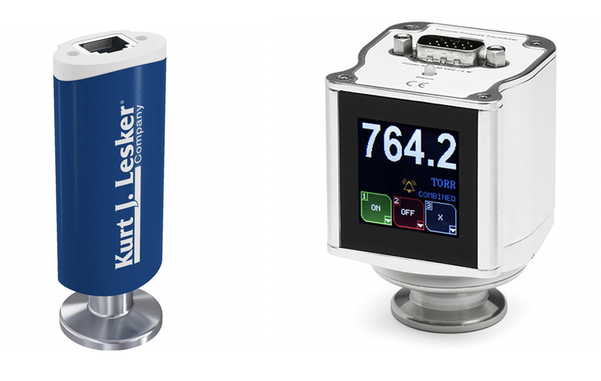
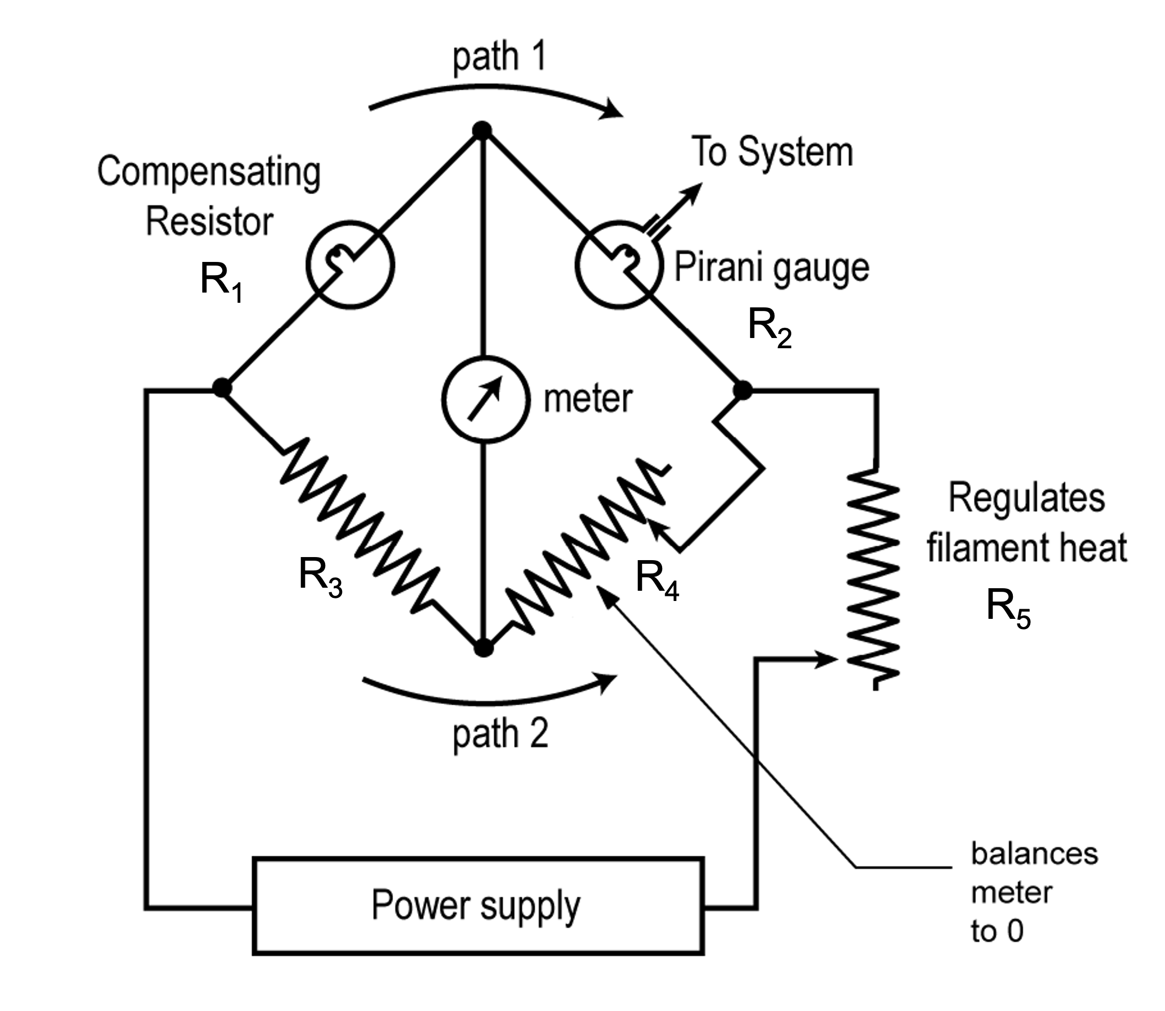
A Pirani gauge, shown in Figure 4.17 is also a type of thermal conductivity gauge. A Pirani gauge consists of a length of thin filament wire that is heated and passed through a metal cylindrical tube. The filament is incorporated in the gauge as one of the resistive arms in a Wheatstone Bridge. A Wheatstone Bridge in its simplest form consists of four resistances arranged in a square, or diamond, shape, like a baseball diamond. Using the baseball analogy, a meter is placed between first base and third base, and a power supply is connected between home plate and second base. As the pressure changes, the Pirani gauge detects a change in an electrical property due to changes in the resistance of the heated filament.
The circuit, shown in Figure 4.18 (a) operates in the following manner. If the bridge is balanced, the voltage at first base equals the voltage at third base, and there is no voltage potential across the meter. No voltage means no current flows through the meter and the meter reads zero. If one of the resistances changes, the bridge will become unbalanced. For example, when pressure in the chamber decreases, the filament within the Pirani transducer heats up, which in turn causes an increase in the filament’s resistance. Then, the voltage at first base and third base will no longer be equal, and the potential difference across the meter will cause an electrical current to flow through the meter. The magnitude of the electrical current will be proportional to the new pressure in the vacuum chamber.
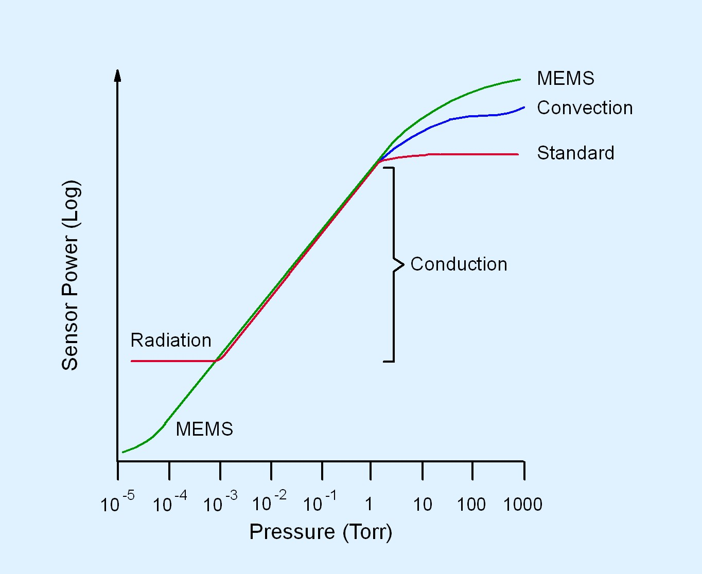
There are two primary Pirani gauge hot-filament designs. One design is based on supplying a constant voltage across the bridge. The pressure is determined by measuring changes in the bridge current caused by changes in the resistance of the filament wire. The constant voltage Pirani gauge design supports pressure measurements in a range of approximately 0.001 to 1 Torr. The second design is based on maintaining a constant filament temperature by adjusting the bridge voltage. The pressure is determined by measuring the changes in power supplied to maintain the constant filament temperature. The constant temperature gauge design supports a measurement range of approximately 0.001 to 100 Torr.
Two other types of Pirani gauge designs are commonly used in vacuum systems. One of them is called the convection-enhanced or convection Pirani gauge. The core design of a convection-enhanced Pirani gauge is the same as the constant filament temperature design. This gauge design is enhanced to provide pressure measurements higher than 100 Torr by utilizing the convection currents around the filament. Figure 4.18 (b) shows that convection becomes the primary heat transfer mechanism for pressures above 10 Torr. The orientation of a convection-enhanced Pirani gauge is critical to its operation. The heated filament must be oriented in a horizontal position. When the gas molecules within the metal tube are in viscous flow, that is, at pressures greater than 10 Torr, convection currents will draw heat from the filament making higher pressure measurements possible. A convection-enhanced Pirani gauge supports a measurement range of approximately 0.001 to 1000 Torr.
The second Pirani gauge design is a significant departure from the heated filament design. This Pirani gauge design is called a MEMS (microelectromechanical systems) Pirani. A MEMS Pirani gauge incorporates the same elements present in the heated filament-based design, but all the elements are fabricated on a silicon substrate as part of a MEMS sensor unit. The function of the heated filament is accomplished by a thin serpentine configuration of nickel metal fabricated on the MEMS sensor. The nickel metal on the MEMS sensor serves as the heated element. The MEMS Pirani gauge supports an extended pressure measurement range from 1 x 10⁻⁵ to 1000 Torr, as shown in Figure 4.18 (c), due to the miniaturized MEMS sensor design.
Measurement accuracy of a specified gas in a properly calibrated hot-filament Pirani gauge is approximately ±10% over the measurement range of 0.001 to 10 Torr. In contrast, properly calibrated convection-enhanced Pirani gauges have a measurement accuracy of ±10% below 10 Torr and ±5% for pressure measurements above 10 Torr. A MEMS Pirani gauge has varying measurement accuracies across its measurement range. At the lowest end, that is, at pressures between 1 x 10⁻⁵ to 1 x 10⁻³ Torr, the measurement accuracy of a MEMS Pirani gauge is ±10%. For pressure measurements between 1 x 10⁻³ to 100 Torr, the measurement accuracy of a MEMS Pirani gauge is ±5%. For pressure measurements above 100 Torr, the MEMS Pirani gauge has a measurement accuracy of ±25%. Pirani gauges can be calibrated at both ends of the measurement range. Pirani gauges provide better measurement accuracy than thermocouple gauges but are not as accurate as capacitance manometer gauges. A convection-enhanced Pirani or a MEMS Pirani gauge will support a much wider measurement range than a capacitance manometer. Pirani gauges are more expensive than thermocouple gauges but much less expensive than a capacitance manometer.
4.5.3.3 Thermal Conductivity Gauges and Gas Species Dependencies
Using a thermal conductivity gauge is not as simple as hooking up the gauge to the vacuum chamber or lines in a vacuum system and reading the numbers off the gauge controller. Since the thermal conductivity of different gases varies, the number representing the pressure may have to be adjusted if the gas composition is different from the gas composition for which the gauge was calibrated. Table 4.2 gives the thermal conductivity of common gases.
Table 4.2. Thermal conductivity of common gases.
|
Gas |
Thermal conductivity MJ/(s · m · K) |
|---|---|
|
Air |
24.0 |
|
Argon |
16.6 |
|
Carbon Dioxide |
14.58 |
|
Helium |
142.0 |
|
Hydrogen |
173.0 |
|
Methane |
30.6 |
|
Neon |
45.5 |
|
Nitrogen |
24.0 |
|
Oxygen |
24.5 |
|
Water Vapor |
24.1 |
|
Xenon |
4.50 |
What Table 4.2 tells us is that the amount of heat lost from the filament in a thermal conductivity gauge depends on the gas(es) in the system. For example, if the chamber is filled with helium as opposed to nitrogen, the helium, having a higher thermal conductivity, will carry more heat away from the filament than nitrogen, and thus an equivalent amount of helium will cool the filament to a greater extent than nitrogen. Argon, on the other hand, with a lower thermal conductivity, will not cool the filament as fast as nitrogen. Figure 4.19 (a) shows heat transfer characteristics of helium, nitrogen and argon depending on pressure. So with any gas other than nitrogen, you should not take the observed pressure reading at face value.

Let’s use the Model PG 105 Convection-Enhanced Pirani gauge produced by Stanford Research Systems (SRS) as an example. All PG 105 gauges are factory-calibrated and temperature-compensated for nitrogen (essentially air). The response of the gauge is very well characterized, and with proper calibration data, it is possible to obtain accurate pressure measurements for other gases as well. For user convenience, nitrogen- and argon-specific calibration curves are loaded into SRS’s Model IGC 100 Gauge Controller, making direct measurements possible for these gases. For other gases, gas-correction curves are provided for the PG 105 gauge (see Figure 4.19 (b) and Figure 4.19 (c)). However, for gases, or mixtures of gases, not included in the gauge data sheet, users will have to generate their own conversion curves.
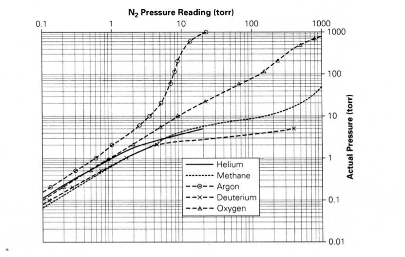
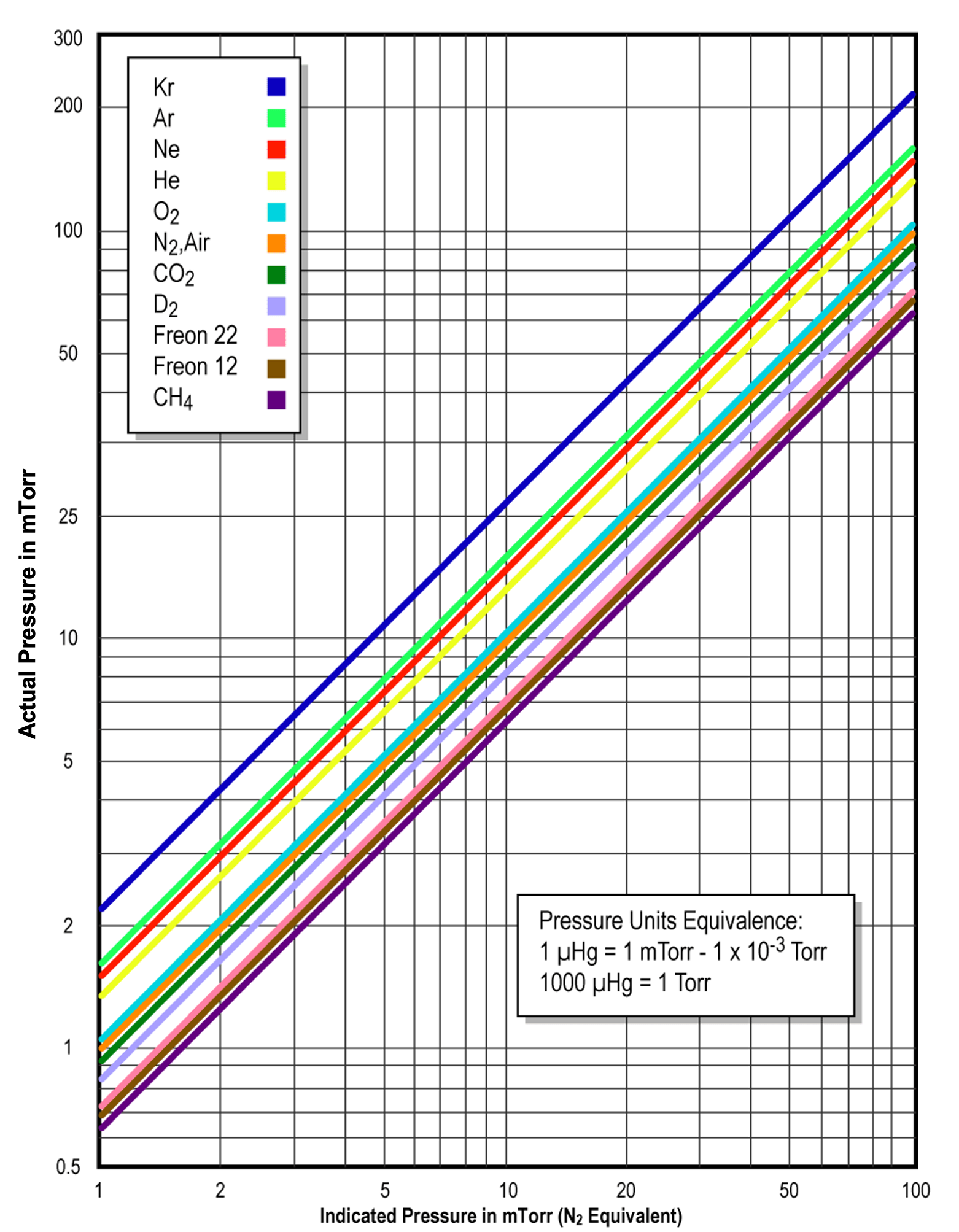
For the PG 105 convection-enhanced Pirani gauge, the actual pressure is equal to the nitrogen-equivalent reading from the gauge controller times the gas-correction factor. For pressures below 1 Torr, the gas correction factor for argon is given as 1.59 in the data sheet. Hence, if the pressure reading on the controller display is 0.50 Torr (the nitrogen equivalent reading), then the actual pressure is equal to 0.50 Torr x 1.59, or approximately 0.80 Torr. When properly configured, controllers such as the Model IGC 100 can perform this calculation for you and display the actual argon pressure on the controller readout. Care should be taken if a thermal conduction gauge calibrated for N2 is present when a vacuum system is vented with argon. The thermal conduction gauge will indicate a lower pressure value than the actual system pressure. The risk would be creating an over-pressure condition if the pressure within the chamber is unknowingly allowed to exceed atmospheric pressure.
On the other hand, if the vacuum chamber is filled with methane and the observed pressure reading on the gauge controller is 0.50 Torr, we can use the given gas-correction figure for methane to determine the actual pressure. From the sensitivity correction data sheet provided with the Model IGC 100 Controller, the gas-correction factor for methane is 0.63. Multiplying the gas-correction factor, 0.63, times the gauge pressure reading, 0.50 Torr, we obtain 0.32 Torr, the actual pressure for methane in the chamber.
It is important to read the operating instructions and data sheet for the pressure gauge you are using. In some cases, you may be instructed to divide (not multiply) the observed reading by the gas-correction factor.
4.5.4 Other Rough Vacuum Gauges
Two other vacuum measurement gauges are worth mentioning. The first one, the piezoelectric vacuum gauge, is another type of direct pressure measurement device. Piezoelectricity is a phenomenon in which electric charge builds up in certain materials as a direct response to a mechanical stress applied to the material. A piezoelectric vacuum gauge includes a piezoelectric sensing unit. This gauge detects changes in an electrical property, for example, resistance, due to material deformation as a response to changes in pressure. A measurement based on the changing electrical property is converted to a pressure reading. Piezoelectric vacuum gauges support a measurement range of 0.1 to 1000 Torr. The measurement accuracy of a piezoelectric vacuum gauge varies over its range of measurement. The accuracy of the measurement is generally 1% or better for pressures of 10 Torr and higher. At pressures below 10 Torr, this device becomes increasingly less accurate.
The other vacuum measurement gauge we will address here is the combination gauge. As the name suggests, this gauge is the combination of two different measurement technologies within a single package. The underlying technologies combined in one unit are the capacitance manometer and Pirani technologies or the piezoelectric and Pirani technologies. A combination gauge can support a measurement range of 1×10⁻⁵ to 1000 Torr. The accuracy of the measurement varies over the device’s measurement range and corresponds to the accuracy of the underlying technology. For the range in which the capacitance manometer or piezoelectric technology applies, the measurement accuracy is better than 1%. For the range in which the Pirani technology applies, the measurement accuracy is 5-10%. The advantage of using a combination gauge is the ability to measure the system pressure over the entire rough vacuum regime using a single device.
Table 4.3. Summary of rough vacuum gauges.
|
Gauge Technology |
Accuracy |
Pressure Range |
Direct vs Indirect |
Response Time |
|---|---|---|---|---|
|
Bourdon |
± 10% |
1 Torr to 760 Torr |
Direct |
Fast (immediate) |
|
Capacitance Diaphragm |
± 0.25% |
Approximately 1.0×10⁻⁴ Torr to 1,000 Torr |
Direct |
Fast (msec) |
|
Thermocouple |
± 15% |
Approximately 0.01 Torr to 1 Torr |
Indirect |
|
|
Pirani (hot filament) |
± 10% |
0.001 Torr to 1 Torr (constant voltage); 0.001 Torr to 100 Torr (constant temperature) |
Indirect |
1 – 2 sec for constant voltage; <50msec for constant temperature |
|
Convection-enhanced Pirani |
± 10% below 10 Torr; ± 5% above 10 Torr |
0.001 Torr to 1,000 Torr |
Indirect |
<50msec in conduction regime; slower in convection regime |
|
MEMs Pirani |
± 10% between 1×10⁻⁵ Torr and 1×10⁻³ Torr; ± 5% between 1×10⁻³ Torr and 100 Torr; ± 25% above 100 Torr |
1.0×10⁻⁵ Torr to 1,000 Torr |
Indirect |
|
4.6 Piping, Valves and Fittings
Other components are needed to configure a suitable and operational vacuum system. The selection of an appropriately sized vacuum chamber is the first consideration. Piping hardware connects the pump to the chamber. A valve is typically inserted in the piping line between the chamber and the pump, so the chamber can be isolated from the pump. Another valve is present and used for venting the chamber to atmosphere. One or more pressure gauges may be connected to the vacuum system to monitor the pressure at critical locations within the system.
At pressures above 10 milliTorr, gas molecules act much like a fluid. We can use our familiarity with the flow of liquids to help us visualize how gas flows in a vacuum system in the rough vacuum regime. Flow in this pressure regime is known as viscous flow. The term “viscous” implies that the gas molecules are “thick”, which also suggests that the number of gas molecules present is very, very large. In viscous flow, the gas molecules are constantly bumping into each other and the walls of the chamber. In fact, the molecules are so closely packed that when some of them are pumped out of the chamber, other gas molecules will rush to fill the empty space and distribute themselves within the chamber. Molecular movement is very predictable in the rough vacuum regime when the flow of the molecules is viscous. Because of this predictability, smaller-diameter hoses and pipes can be used when large quantities of molecules per unit time move from one place in the system to another.
In the rough vacuum regime, a variety of options are available for the piping that connects the system components. In a vacuum system with a base pressure of 10 milliTorr or higher, it is reasonable to use piping made of materials such as plastics and elastomers. For example, flexible polyvinyl chloride (PVC) cord-reinforced vacuum hose is a very suitable piping for connecting a positive displacement vacuum pump to a chamber. Gaskets made out of elastomer materials have elastic qualities making them reusable. Elastomer gaskets are used at demountable junctions in vacuum systems. However, plastics and elastomers are not suitable materials to use in vacuum chambers and piping that are required to establish and maintain high vacuum conditions. Plastic and elastomer type materials have relatively high vapor pressures and high permeability rates. These materials adversely contribute to the gas load in a vacuum system through outgassing and permeation. The presence of elastomer chamber materials will make it difficult or impossible for a system to attain a base pressure in high vacuum. In a manufacturing setting and for vacuum systems with base pressures in the high vacuum regime, the piping is usually made of stainless steel or aluminum.
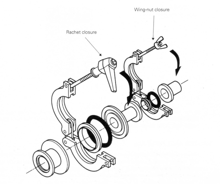
Klein Flansche flanges (KF flanges) are common classes of vacuum flanges and fittings used in the rough vacuum regime. As shown in Figure 4.20, KF flanges use a centering ring with an elastomer O-ring as the seal. The O-rings are made of either Buna-N or Viton. These particular elastomer materials have low outgassing rates. The O-ring is placed within a centering ring which is then positioned between the two components to be joined. A clamp is then used to hold the two components together and compress the elastomer O-ring to form a good seal. Flanges come in standard sizes ranging from KF10, the smallest, to KF50, the largest size. The KF10 is used to connect a tube of 10 mm inside diameter (ID), while the KF50 connects to a tube of 50 mm ID.
When using KF flanges to make a connection, it is important to ensure that the groove and mating surface are clean and dry. Check the sealing surfaces for scratches that cross the sealing area. If O-rings are reused, visually inspect them to make sure they do not have small crosswise cracks or nicks that might leak. Since elastomer material is very permeable, greases and solvents should be used on elastomer seals in a vacuum system sparingly or not at all. Greases and solvents that permeate into the elastomer O-ring will outgas into the vacuum system. When grease is applied to an O-ring, it should be one with a low vapor pressure. If an O-ring has been exposed to solvents or excessive heat that has caused it to swell or deform, do not reuse it. Replace it with a new one.
Valves are used to provide isolation between vacuum components. The block valve is commonly used for this purpose in the rough vacuum regime. Block valves are made of aluminum, stainless steel, or brass. They can either be hand-operated, pneumatically (air)-operated, or activated electromagnetically. Flange options include KF flanges as well as others. They can be either in-line or right-angle. Figure 4.21 shows some examples of various metal valves with KF flanges.

KF fittings include nipples, elbows, tees, and reducers, to name a few. Figure 4.22 shows some of these KF fittings.

And finally, we need a valve that we can use to vent the system back to atmospheric pressure. Metal sealed or elastomer-sealed valves can be used for this purpose. They can also be used as gas inlets for process gases to the process chamber.
4.7 Rough Vacuum Pump-Down Process
To pump down the vacuum chamber in our simple rough vacuum system shown in Figure 4.1, the following procedure can be used. Let’s assume that the vent valve and roughing valve are both closed and the chamber is filled with air at atmospheric pressure. If we are operating a system at a location near sea level, the rough vacuum gauge will be calibrated to display a reading very close to 760 Torr.
Prior to beginning the pump-down process, the rough vacuum pump is started and the roughing line between the pump and the rough vacuum valve pumps down. If this volume between the pump and the roughing valve is small, the pump-down time should be very short. To start the chamber pump-down process, the roughing valve is opened. The vacuum pump repetitively captures volumes of air from within the system including the chamber and expels those trapped gas molecules to the surrounding atmosphere. The molecular density within the chamber decreases as the quantity of molecules present within the chamber volume decreases. The pressure gauge will sense the decreasing molecular density condition in the chamber and will indicate a decreasing pressure reading on the pressure display. It should be noted that a convection-enhanced Pirani gauge may initially show an increase in pressure before it shows the pressure starting to decrease. The pressure in a small chamber will drop quickly and then gradually level off at the base pressure of the system. The pump-down time for the system will depend on the size of the gas load and the net pumping speed of the rough vacuum system. Figure 4.23 shows the general shape of the pressure versus time graph for a rough vacuum system.

For pressures above 0.01 Torr (10 mTorr), the volume of the chamber and pumping speed are the determining factors when calculating pump-down times. Let’s assume that we have a chamber of volume V with a pump connected directly to the chamber that achieves an effective pumping speed Seff. The ultimate pressure of the pump is specified as Pult. At time t = 0, the initial pressure shall be Pi . The pump-down time from Pi to some final pressure Pf (Pf > Pult) can be estimated by
Equation 4.2 assumes that the chamber is clean and does not have any leaks. It also assumes that the conductance of the connection between the pump and the chamber is much greater than the effective pumping speed of the pump.
Equation 4.3 implies that the pressure versus time curve follows an exponential decay of the form,
In Equation 4.3, Pf of Equation 4.2 is replaced with the more general term p(t), where p(t) means pressure as a function of time.
Example 4.7
A rotary vane pump with a nominal pumping speed of 193 liters per minute is used to pump down a 300-liter chamber. How long will it take to pump down the chamber from atmosphere to 1 Torr? Assume the pump connects directly to the chamber and the conductance of the connection between the pump and the chamber is much greater than the effective pumping speed of the pump. Assume that from the data sheet, the pump’s ultimate vacuum pressure, Pult, is 0.003 Torr.
Solution:
From the problem statement, we are given the volume of the chamber, V, as 300 liters, the effective pumping speed, Seff, as 193 liters per minute, the starting pressure, Pi, as atmospheric pressure, which is assumed to be 760 Torr, and the final pressure, Pf, is 1 Torr.
Substituting this information into Equation 4.2 yields
Since 0.003 Torr is much smaller than 1 Torr, the equation simplifies to
Example 4.8
A mechanical diaphragm pump with a nominal pumping speed of 40 liters/min is used to evacuate the same 300-liter chamber as in Example 4.7. The pump’s ultimate pressure is 3.8 Torr. How long will it take this pump to reduce the pressure in the chamber from atmosphere to 10 Torr? Assume the pump connects directly to the chamber and the conductance of the connection between the pump and the chamber is much greater than the effective pumping speed of the pump.
Solution:
From the problem statement, the volume of the chamber, V, is 300 liters, the initial pressure, Pi, is atmospheric pressure and assumed to be 760 Torr, and the final pressure, Pf, is 10 Torr. The nominal pumping speed is 40 liters per minute, and the ultimate vacuum pressure, Pult, is 3.8 Torr.
Substituting this information into Equation 4.2 yields
Performing the computations yields
Note: In this case the vacuum pump’s ultimate pressure is significant. If the ultimate pressure value is assumed to be negligible, the pump-down calculation yields 32 minutes, about a 10% difference.
Example 4.9
Calculate the pump-down time for the Anest Iwata ISP-90 Oil-Free Scroll Mechanical Vacuum Pump to reduce the pressure in a 13.0-liter chamber from atmosphere (105 Pa) to 10 Pa. Use the pump speed curve for the ISP-90 shown in Figure 4.24.a. Assume the pump connects directly to the chamber and the conductance of the connection between the pump and the chamber is much greater than the effective pumping speed of the pump.
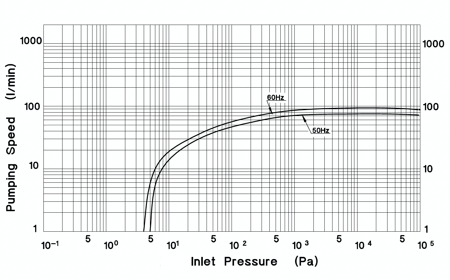
Solution:
From the ISP-90 pumping speed curve, we observe that the pumping speed is approximately 93 liters/min from atmosphere to about 1000 Pa. Below 1000 Pa, the pumping speed rolls off with a slope of 3.6 liters/min per decade of pressure. If we assume that the pumping speed is constant at 93 liters/min over the entire pressure range from atmosphere to 10 Pa, our calculated pump-down time will be shorter than the actual pump-down time. Therefore, we need a better method for calculating the pump-down time.
One alternative method is to use a piece-wise linear approximation for the pumping speed curve. To implement this method, let us divide the pressure range into two segments. To do this, we need to plot two lines on the pump speed curve. The first line will be horizontal and tangent to the speed curve for pressures above 1000 Pa. The second line will be tangent to the sloped curve somewhere between 10 Pa and 1000 Pa depending on how conservative we want to approximate the pump-down time. The point where these two lines cross (as shown in Figure 4.24.b) will determine the pressure (300 Pa) separating the two pressure segments. Thus, the first pressure segment is from atmosphere (105 Pa) to 300 Pa, where the pumping speed is a constant 93 liters/min as read from the graph. And the second range is from 300 Pa to 10 Pa, where the pumping speed decreases from 93 liters/min to approximately 20 liters/min at 10 Pa. We can find an average pumping speed in the 300 Pa to 10 Pa range by adding 93 liters/min and 20 liters/min and dividing by 2 (essentially finding the average pumping speed over this pressure range). This yields an average pumping speed over this range of 56.5 liters/min. Now we can calculate the pump-down time for each pressure segment and then add both time segments to find the total pump-down time.
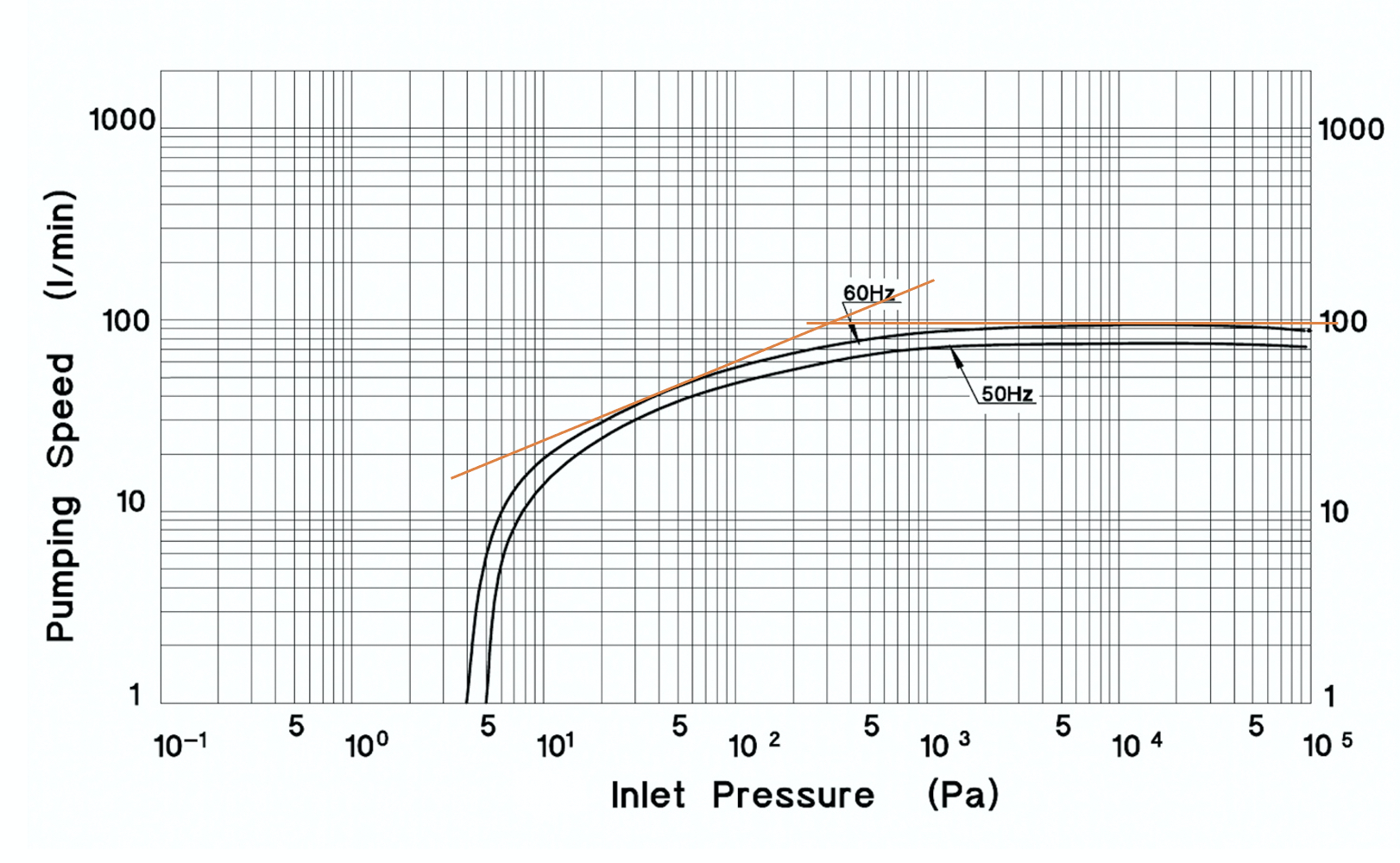
using ISP-90 oil-free scroll mechanical pump speed curve.
How does this compare to the pump-down time using the assumption that the pumping speed is a constant 93 liters/min over the entire pressure range? The pump-down calculation using the constant 93 liters/min pumping speed yields a pump-down time of 1.36 minutes, a difference of 0.35 minutes or 20.5%. Is this significant? It depends on the application. Purely from a time perspective, a 20.5% difference can seem substantial. But for this particular result, the pump-down time is so short that it may not make much of a noticeable difference when operating the system.
4.8 Conductance
But wait a minute. What about the effect of the piping if the rough pump has to be placed at some distance from the vacuum chamber? Wouldn’t it affect the pump’s ability to remove gas from the chamber? The answer is, “It depends.”
From our experience in daily life, we know that pipes, or tubes, of varying lengths and cross-sections can conduct gases and liquids with different degrees of difficulty. Say, you are drinking a soft drink through a straw. Drawing the liquid through a regular 8-inch straw poses no great difficulty. Now, imagine that the straw is 30 inches long. It would take more effort to drink the liquid if one had to draw it along the entire length of the straw. Or imagine that an 8-inch straw of one-tenth the diameter is used. It would again require more effort to draw the liquid through the narrower straw.
The ease with which a gas or liquid is drawn through a pathway of given geometry is quantified by a property called conductance. Conductance values depend not only on the pressure and the nature of the gas flow, but also on the shape of the conducting element. Other factors are the conducting element’s length and whether it is straight or curved. The result is a large set of equations that take into account various combinations of these elements that affect conductance.
For example, the conductance of a straight pipe, or tube, Ct, shown in Figure 4.25, of length L and with a circular cross-section of diameter d, operating in the laminar flow range, is given by
where
Ct is the conductance in liters per second,
d is the cross-sectional diameter of the pipe in centimeters,
L is the length of the pipe in centimeters, and
pave is the average pressure in the pipe in torr,
where p1 is the pressure at the start of the pipe (along the direction of flow) and p2 is the pressure at the end of the pipe.
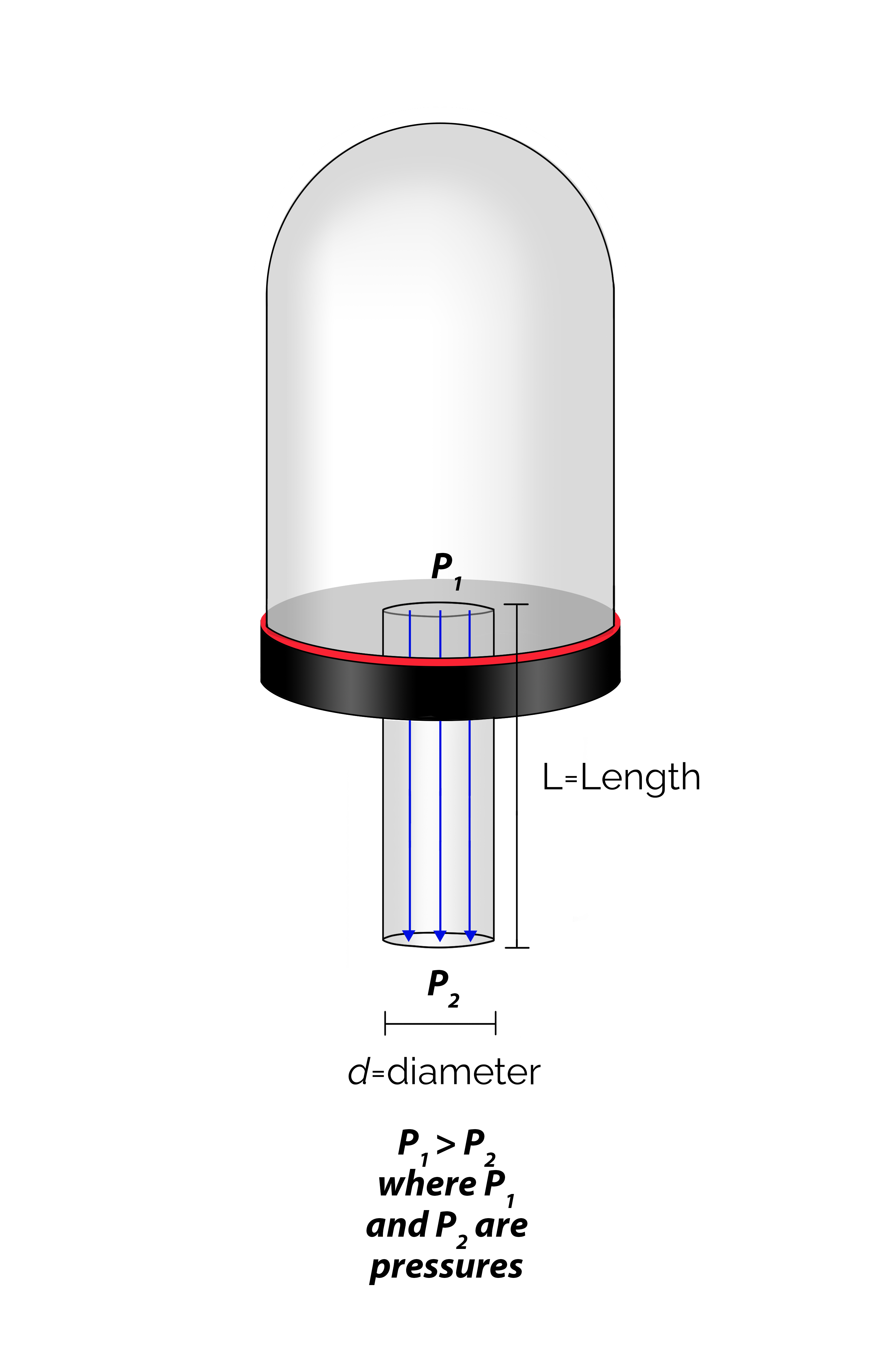
Example 4.10
What is the conductance of a 15-inch long pipe with an inside diameter (ID) of 0.5 inches if the pressure is 20 Torr at the start of the pipe and 1 Torr at the end of the pipe? Assume that the gas flow within the pipe is viscous laminar.
Solution:
We are given the following information:
pave can be calculated from the pressures at the ends of the pipe:
Substituting these value into Equation 4.4 yields,
We now ask a follow-up question: Is there a conductance at the aperture where the gas enters the pipe from the chamber? (See Figure 4.26.) There certainly seems to be some congestion occurring here, much like the masses of people leaving a football stadium at the end of the game.
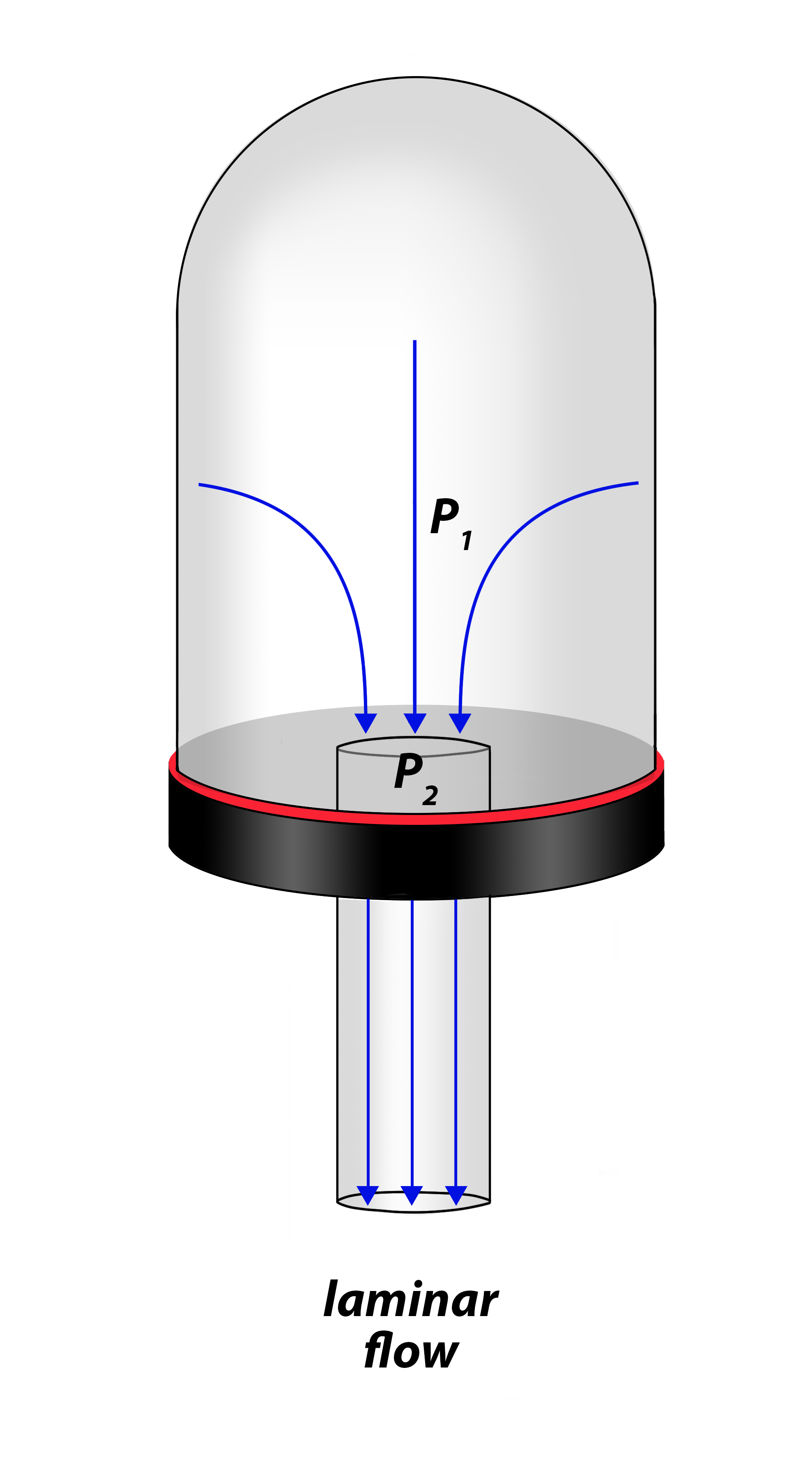
For viscous flow, the conductance of the aperture can be calculated using the following equation,
where
Ca is the conductance of the aperture in liter per second,
A is the cross-sectional area of the aperture in cm2, and
δ is the ratio of P2 to P1 where P2 is the pressure in the pipe and P1 is the pressure in the chamber (for the gas to flow out of the chamber and through the pipe to the pump in the system, P1 must be greater than P2).
But, are we in viscous flow? The following condition, based on the ultimate pressure, Pu, and the cross-sectional diameter, d, of the circular pipe, can be used,
For the preceding example, the ultimate pressure was 1 Torr and the diameter of the pipe was 1.27 cm. Applying the test for viscous flow,
Thus, the condition for viscous flow is met, and Equation 4.5 can be used.
Note that in the viscous flow, δ is usually very small and Equation 4.5 reduces to
As a result, in the viscous flow range, the conductance is not a function of pressure, but only depends on the geometry of the aperture.
Returning to our Example 4.10, we can determine the conductance of an aperture of diameter 0.5 inches, or 1.27 cm. Using Equation 4.6 yields,
Since the conductance of the tube and the conductance of the aperture act as series elements, the two conductances can be combined as follows:
or
Substituting our values for our 15-inch long pipe with 0.5-inch diameter yields a net conductance of
The final step is to calculate the net pumping speed by combining the net conductance of the piping and the pump’s speed in series. This has the same form as Equation 3.3.
where
Snet is the net conductance or pumping speed of the pump plus the piping,
Cnet is the net conductance of the piping, and
Sp is the pumping speed of the vacuum pump.
Equation 4.9 can be rearranged and an equation for Snet can be written,
Example 4.11
What is the net pumping speed at the outlet of the vacuum chamber if a 90-liter-per-minute mechanical pump is connected to piping in Example 4.10? Give the net pumping speed in liters per second. Assume that viscous flow conditions apply.
Solution:
Since the net pumping speed is to be specified in liters per second, the pumping speed of the mechanical pump should be converted to liters per second.
Substituting the given values for Cnet and Sp into Equation 4.10 yields,
In this example, we note that the conductance of the piping is much greater than the pumping speed of the pump. Therefore, the factor limiting the net pumping speed is the pumping speed of the mechanical pump, not the size of the piping. However, this is not always the case.
4.9 Troubleshooting Rough Vacuum Systems
There are a number of things that can go wrong with rough vacuum systems. Knowing the optimal behavior of your vacuum system when it is functioning properly helps in detecting and troubleshooting system problems when they occur. This section discusses some common problems and how to fix them.
4.9.1 No Start-Up
Failure to start up is one of the simpler things to diagnose and possibly to fix. The observed symptom is the failure of the mechanical pump to start when the power is turned on. The cause may be that power is not getting to the pump. Corrective action begins with checking the electrical system. This includes checking the power switch to see if it is actually in the ON position, checking the circuit breaker, which may have been switched OFF. Another possibility is an open circuit in the power line running to the pump. A voltmeter can be used to measure the voltage at the pump.
Another possibility is that the pump has frozen or seized up. In this case, the observed symptom may be a whining or buzzing noise indicating that the motor is trying to turn but cannot do so for some reason. If this condition persists, overheating may be detected by a burning odor.
4.9.2 Pump is running, but no vacuum is detected
If the pump is operating normally, but the system pressure does not decrease, there are several possible causes. If the mechanical pump uses a belt drive, it is possible that the belt has broken or slipped off the pulley(s). Another possibility is that the rough valve has not been opened. A third possibility is that the vent valve has not been closed and is in the open position. Another possibility is another very large leak to atmosphere exists somewhere in the system.
It is also possible that an accurate pressure reading is not being displayed. If a multi-gauge controller is being used, it may be displaying a reading from the wrong gauge, a gauge in another part of the vacuum system that is looking at atmospheric pressure.
4.9.3 Deviation from standard pump-down curve
A deviation from the standard pump-down curve can be caused by an increase in the gas load or a change in the characteristics of the pressure gauge. Increases in the gas load can be caused by leaks in the system or the presence of one or more contaminants in the system or in the vacuum pump, such as condensed water vapor, solvents, or gases in the pump oil.
Pressure readings that are too high, or too low, can be caused by a dirty or contaminated sensor.
4.9.4 Cannot reach base pressure
Failure to reach base pressure can be caused by an increase in gas load or a problem within the pump. Increased gas load often results from a leak, but this is not the only cause. Contamination can also increase the gas load significantly and adversely impact the system’s ability to achieve base pressure. The most significant contaminant to be mindful of in rough vacuum as well as high vacuum is water vapor.
A drift in the performance of the pressure gauge can also be the cause of a perceived change in the base pressure level attained by the system. In addition, if system’s chamber originally contains gas other than air (for example, argon), then direct-reading gauges and indirect-reading gauges will display different values.
Summary
Rough vacuum systems are relatively simple and minimally consist of a single mechanical pump, chamber, and pressure gauge, one or more valves, and piping. The types of mechanical pumps used include rotary vane and piston pumps, diaphragm pumps, and scroll pumps. These pumps operate by expanding the volume, trapping a volume of gas, compressing the gas, and finally exhausting the gas from the pump. Pump selection will depend on the application, cost, pumping speed requirements, and space, among other factors.
Vacuum gauges used in rough vacuum systems can be either direct-reading pressure gauges like capacitance manometers or indirect-reading pressure gauges like thermocouple and Pirani gauges. Pressure gauge selection will be influenced by such factors as cost, pressure range, and response time. It is important to remember that thermal conductivity gauges are sensitive to gas type. They are calibrated for nitrogen, but gauge readings for other gases require correction using the correction factors supplied with the pressure gauge. Direct-reading pressure gauge readings do not require correction for gas type.
A wide variety of fittings can be used in rough vacuum systems. KF fittings are the most common ones used in rough vacuum regime. Piping can be made of flexible plastic materials or metals. Again, it depends on the application, cost constraints, and other factors relevant to your application.
Graphing the rough vacuum pump-down curves for your vacuum system will help characterize and establish the nominal performance of your rough vacuum system. By comparing present pump-down curves to past pump-down curves, you can detect changes in system performance and take corrective action, if necessary.
Maintaining rough vacuum systems is relatively easy. Mechanical vacuum pumps require regular maintenance to replace seals and diaphragms and change pump oil. Chambers may require periodic cleaning, depending on what is being pumped.
Troubleshooting rough vacuum systems usually focuses on leaks and worn-out system components. Failure of the vacuum system to pump down to base pressure can be caused by leaks, failure to open the roughing valve, failure to close a manual vent valve, failure of an automatic vent valve to close, or an error with the gauge operation. It can also be caused by wear on system components and may indicate the need for system maintenance to replace worn-out components.
References
Basic Vacuum Practice. 3rd Edition, Varian Vacuum Products, Lexington, MA 1992.
Borichevsky, Steve. Understanding Modern Vacuum Technology. Blue Dasher, Ipswich, MA, 2017.
Hansen, Steve. “Boyle’s Law and the Pump Down: Incremental Vacuum.” Vacuum Technology & Coating, July 2011.
Hansen, Steve. “Going to Extremes: Exploring the Upper and Lower Bounds of the Pirani Gauge’s Response.” Vacuum Technology & Coating, May 2012, pp. 14–17.
Harris, Nigel. Modern Vacuum Practice. 3rd Edition, Nigel S. Harris, 2007.
Hoffman, Dorothy M., Singh, Bawa, and Thomas, John H., III, Editors. Handbook of Vacuum Science and Technology. Academic Press, 1998.
HPS Products Series #25 Moducell: Pirani Vacuum Sensor/Transducer Operation and Maintenance Manual. MKS Instruments, Wilmington, MA, 1999.
HPS Products Series 907: Analog Convection Transducer (ACT) Vacuum Sensor Operation and Maintenance Manual. MKS Instruments, Wilmington, MA, 1999.
Introduction to Vacuum Gauging Techniques. MKS Instruments, Wilmington, MA, 1998.
Jousten, K. Handbook of Vacuum Technology / Edited by Karl Jousten. Second, completely revised and updated edition., Wiley-VCH Verlag GmbH & Co. KGaA, 2016.
Lafferty. J. M., Editor. Foundation of Vacuum Science and Technology. 3rd Edition, Wiley Interscience, Hoboken, NJ, 2003.
O’Hanlon, John. A User’s Guide to Vacuum Technology. 3rd Edition, Wiley Interscience, Hoboken, NJ, 2003.
Questions and Problems
- A 0.50-liter piston pump is connected to a 5-liter chamber. Assume that the pressure in the chamber is atmospheric pressure (1 atm). What will be the pressure in the chamber after eight strokes of the piston pump?
- A 0.25-liter piston pump is connected to a 20-liter chamber. How many strokes of the piston pump will be needed to reduce the pressure in the chamber from one atmosphere to 0.75 atmospheres?
- A diaphragm pump is connected to a cylindrical chamber 15-inches in diameter and 12 inches in length. How long will it take the pump to reduce the pressure in the chamber from atmosphere to 10 Torr? Assume the nominal pumping speed of the pump is 30 liters per minute, the ultimate vacuum pressure, Pult, is 1.2 Torr, and the piping from the pump to the chamber is not a limiting factor.
- A Varian SD-451 mechanical pump is connected to a 200-liter chamber. Assuming that the conductance of the connecting pipe is not a limiting factor, how long will it take to pump down the chamber from atmosphere to 0.5 Torr? Show all calculation and list all assumptions made. Use the following pump specs for your calculations if necessary: nominal pumping speed 14.6 cfm, ultimate pressure 1.5 x 10⁻³ Torr.
- Calculate the pump-down time for an IDP-7 Dry Scroll Mechanical Vacuum Pump to reduce the pressure in a 450.0-liter chamber from atmosphere to 1 Torr. Use the pump speed curve for the IDP-7 shown in Figure 4.27. Assume that pump connects directly to the chamber and the conductance of the connection between the pump and the chamber is much greater than the effective pumping speed of the pump.
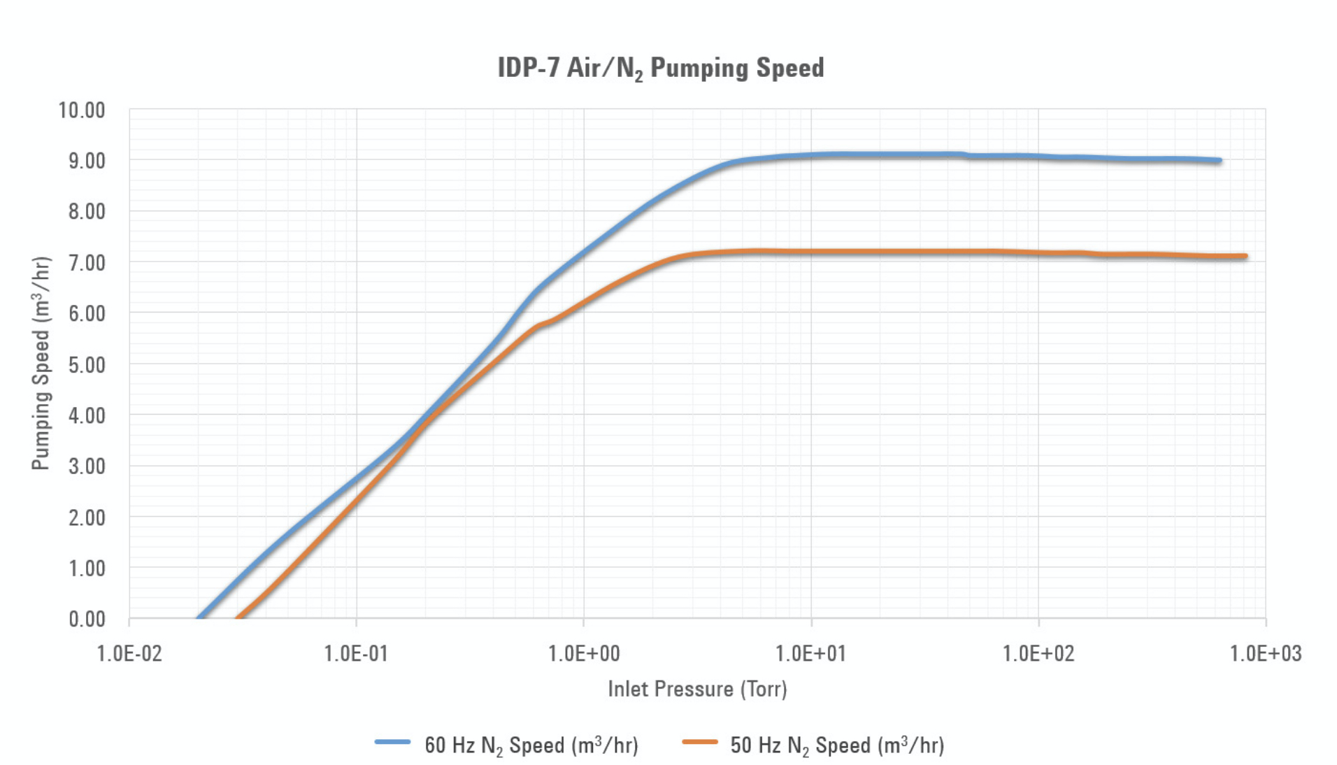
Figure 4.27. Pumping speed curve for IDP-7 dry scroll vacuum pump. Source: Kurt J. Lesker Company, https://www.lesker.com/newweb/vacuum_pumps/pdf/manuals/agilentvarian-idp7-manual.pdf. - Three identical thermal conductivity gauges are used to measure the gas pressure in three identical tanks of equal volume. Each tank contains the same number of moles of gas. Tank 1 contains dry nitrogen gas, Tank 2 contains argon gas, and Tank 3 contains helium gas. Which gauge will read the highest pressure, and why? Which tank will read the lowest pressure and why?
- Determine the net conductance of a circular pipe 25 cm long and 3.0 cm in diameter if the pressure at one end of the pipe is 30 Torr and at the other end is 4 Torr.
- Determine the smallest inside diameter (ID) of the aperture between the chamber and the circular pipe necessary to maintain viscous flow. Assume that system uses the IDP-7 dry scroll pump (Figure 4.27). Then calculate the net conductance of the circular aperture with this ID.
- A 150-liter-per-minute mechanical pump is connected to a 20-inch circular pipe with inside diameter (ID) of 2.0 inches. The pressure in the chamber (and at the start of the pipe) is 80 Torr and 3 Torr at the other end of the pipe. The ultimate pressure of the pump is 0.5 Torr.
- Check if viscous flow condition is met.
- Calculate the conductance of the given circular pipe.
- Calculate the conductance of the given circular aperture.
- Calculate the net pumping speed at the outlet of the vacuum chamber in liters per minute. In liters per second. In m3/hr.
![]()
This work is supported by the National Science Foundation under grant number 2000454. Any opinions, findings, and conclusions or recommendations expressed in this e-book are those of the authors and do not necessarily reflect the views of the National Science Foundation.
Media Attributions
- Figure 4.1. © David Hata is licensed under a CC BY-NC-SA (Attribution NonCommercial ShareAlike) license
- Figure 4.2. © Nancy Louwagie is licensed under a CC BY-NC-SA (Attribution NonCommercial ShareAlike) license
- Figure 4.3. © Nancy Louwagie is licensed under a CC BY-NC-SA (Attribution NonCommercial ShareAlike) license
- Figure 4.4. © Nancy Louwagie is licensed under a CC BY-NC-SA (Attribution NonCommercial ShareAlike) license
- Figure 4.5. © Elena Brewer is licensed under a CC BY-NC-SA (Attribution NonCommercial ShareAlike) license
- Figure 4.6. © MATEC, edited by E.Brewer is licensed under a CC BY-NC-SA (Attribution NonCommercial ShareAlike) license
- Figure 4.7. © Kurt J. Lesker Company is licensed under a CC BY-ND (Attribution NoDerivatives) license
- Figure 4.8. © MATEC, edited by E.Brewer is licensed under a CC BY-NC-SA (Attribution NonCommercial ShareAlike) license
- Figure 4.9. © Kurt J. Lesker Company is licensed under a CC BY-ND (Attribution NoDerivatives) license
- Figure 4.10 (a) © MATEC is licensed under a CC BY-NC-SA (Attribution NonCommercial ShareAlike) license
- Figure 4.10 (b) © MATEC is licensed under a CC BY-NC-SA (Attribution NonCommercial ShareAlike) license
- Figure 4.10 (c) © MATEC adapted by E. Brewer is licensed under a CC BY-NC-SA (Attribution NonCommercial ShareAlike) license
- Figure 4.11. © Kurt J. Lesker Company is licensed under a CC BY-NC-ND (Attribution NonCommercial NoDerivatives) license
- Figure 4.12. © Kurt J. Lesker Company is licensed under a CC BY-ND (Attribution NoDerivatives) license
- Figure 4.13. © MATEC, edited by E.Brewer is licensed under a CC BY-NC-SA (Attribution NonCommercial ShareAlike) license
- Figure 4.14.c. © Gigi Bocek is licensed under a CC BY-NC-SA (Attribution NonCommercial ShareAlike) license
- Fig 4.15 is licensed under a CC BY (Attribution) license
- Figure 4.16 (a) © MATEC is licensed under a CC BY-NC-SA (Attribution NonCommercial ShareAlike) license
- Figure 4.16 (b) © MATEC is licensed under a CC BY-NC-SA (Attribution NonCommercial ShareAlike) license
- Figure 4.17. is licensed under a CC BY-ND (Attribution NoDerivatives) license
- Figure 4.18 (a) © MATEC is licensed under a CC BY-NC-SA (Attribution NonCommercial ShareAlike) license
- Figure 4.18 (b) © MATEC is licensed under a CC BY-NC-SA (Attribution NonCommercial ShareAlike) license
- Figure 4.18 (c) © Steve Hansen is licensed under a CC BY-NC-SA (Attribution NonCommercial ShareAlike) license
- Figure 4.19 (a) © MATEC adapted by E. Brewer is licensed under a CC BY-NC-SA (Attribution NonCommercial ShareAlike) license
- Figure 4.19 (b) is licensed under a CC BY-NC-SA (Attribution NonCommercial ShareAlike) license
- Figure 4.19 (c) © MATEC adapted by E. Brewer is licensed under a CC BY-NC-SA (Attribution NonCommercial ShareAlike) license
- Figure 4.20. © Varian Vacuum Products is licensed under a CC BY-ND (Attribution NoDerivatives) license
- Figure 4.21. is licensed under a CC BY-ND (Attribution NoDerivatives) license
- Figure 4.22. © Rich Hill is licensed under a CC BY-NC-SA (Attribution NonCommercial ShareAlike) license
- Figure 4.23. © Elena Brewer is licensed under a CC BY-NC-SA (Attribution NonCommercial ShareAlike) license
- Figure 4.24.a. is licensed under a CC BY-NC-SA (Attribution NonCommercial ShareAlike) license
- Figure 4.24.b. is licensed under a CC BY-NC-SA (Attribution NonCommercial ShareAlike) license
- Figure 4.25. © Gigi Bocek is licensed under a CC BY-NC-SA (Attribution NonCommercial ShareAlike) license
- Figure 4.26. © Gigi Bocek is licensed under a CC BY-NC-SA (Attribution NonCommercial ShareAlike) license
- Figure 4.27. is licensed under a CC BY-ND (Attribution NoDerivatives) license
The amount of gas that must be removed from the chamber in a vacuum system by the vacuum pump(s). It is typically measured in torr-liters per second, cubic feet per minute, or cubic meters per hour.
The pressure exerted typically by the Earth’s atmosphere. Also see standard atmospheric pressure and standard temperature and pressure (STP).
Vacuum pressure regime with pressures between 760 Torr and 1E-3 Torr.
The number of molecules per unit volume of gas.
The average distance which a molecule travels between two successive collisions with other molecules of the gas.
The volume of gas trapped within the chamber and vacuum piping components prior to initiating a pump-down cycle. Also called volume gas.
A crack, hole, or other pathway that allows gases to pass through from outside the vacuum system to inside the vacuum system.
Graph describing a time-dependent pressure drop in a vacuum system; popular control instrument when designing and operating a vacuum system.
A vacuum component that moves gas molecules from a low-pressure region to a higher-pressure region. Vacuum-pump design is typically specific to its operating-pressure region, with the three main pressure regions being low vacuum (i.e., atmospheric pressure to ~1E-3 Torr), high vacuum (i.e., 1E-3 to1E-9 Torr), and ultra-high vacuum (i.e., less than 1E-9 Torr).
Time required to evacuate a chamber from atmospheric to a predefined base pressure.
Lowest attainable pressure in a vacuum system. In a vacuum pump, the lowest pressure that can be attained with that pump. Ultimate pressure is limited by the pumping speed of the vacuum pump and the vapor pressure of the sealing fluid, among other factors.
Roughing a vacuum chamber indicates that it is being evacuated with a low-vacuum pump through a roughing line from atmospheric pressure to a pressure that is sufficiently low to allow a high vacuum pump to be engaged.
A vacuum pump that draws air by periodically changing the working volume of the pump.
A centralized system within a building to remove exhaust gases from pumps and pumping systems.
One of several types of electrical or mechanical devices used to measure pressure and/or gas density at various locations of a vacuum system.
Part of a vacuum system that controls the flow of outside air (or gas) into the vacuum chamber.
The liberation of gases and vapors sorbed (adsorbed and absorbed) by a material.
A volume of trapped gas that enters the vacuum system when the system is pumped down.
The process of gas molecules that are weakly bound to a surface, bound to pores or cracks in a material, or diffused into the bulk leaving the surface to become gas-phase molecules. Also known as surface desorption.
A process in which atoms or molecules move through a solid, liquid or gas.
The process of molecular penetration of gases, vapors, or fluids completely through a material.
When unwanted gases like oil vapor or particles flow from downstream pumping or other components toward the vacuum chamber or process components, that is, in a direction opposite to the direction of the desired gas flow.
In vacuum systems, mechanical pumps are motor-driven pumps that move gas from the inlet port to outlet port using a mechanical mechanism, e.g. rotary vanes, scrolls, pistons, and diaphragms among others.
A classification of pump that captures a volume of gas near the inlet and mechanically displaces it to the outlet. Often compression of the captured volume occurs between the inlet and the outlet.
A type of positive displacement pump where the high-pressure seal reciprocates with the piston. Also called rotary piston (vacuum) pump.
The temperature at which gas-phase molecules have zero kinetic energy. This value is known as zero degrees Kelvin (0 K) which is approximately -273.15 degrees Celsius.
A type of dry mechanical, rough vacuum pump that utilizes a movable diaphragm element to displace and compress a volume of gas from an inlet to an outlet region.
Vacuum pumps that use no fluids for sealing or momentum transfer.
A rough vacuum pump used in a vacuum system with the inlet of the rough vacuum pump connected to the outlet of a momentum transfer type-high vacuum pump. The rough vacuum pump operates to maintain an effective pressure in the foreline (also called backing line) for the expected throughput.
A dry mechanical vacuum pump design that utilizes two intermeshed spirals (i.e., scrolls) to displace and compress a crescent-shaped volume of gas from an inlet to an outlet region.
A positive-displacement pump that consists of vanes mounted to a rotor that rotates inside a cavity. Invented by Charles C. Barnes in 1874.
A tube that connects the gas outlet from a vacuum system to a building exhaust system.
Generally referring to the condition when gas-phase molecules have adsorbed onto a surface or coalesced within a volume to an extent that this can be visually observed.
The pressure exerted by a vapor which is in thermodynamic equilibrium with one of its condensed phases at the prevailing temperature.
A rotary plunger type pump where two symmetrically shaped impellors rotate in opposite directions inside the pump housing. Roots pumps are used where great volumes have to be pumped. Also known as lobe blower pump.
Claw pumps use two claws rotating in opposite directions, like the Roots pump, to capture, compress, and exhaust the gas. Claw pumps can be used to effectively pump corrosive and abrasive gases. They are often combined with Roots pumps to achieve high pumping speeds and pressures in the millitorr range.
A dry mechanical pump that contains two screw rotors which rotate inside a cylinder. The gas is trapped between cylinder and screw chambers and carried to the gas exhaust.
Pressure gauges that operate by sensing deflection of a solid or liquid surface caused by momentum transfer to that surface from energetic gas molecules. Direct reading gauges are largely insensitive to gas type.
Pressure gauges that measure a property related to gas pressure and then convert that measurement into a gas pressure reading.
A type of direct reading vacuum gauge with a thin-walled metal tube bent into a circular arc that will straighten if pressure is applied to the inside of the tube. The movement of the metal tube is used to indicate pressure. Bourdon gauge was invented by Eugene Bourdon (1808-1884), a brilliant French watchmaker and engineer, in 1849.
The difference between absolute pressure and atmospheric pressure.
Commonly used term for evacuation of a vacuum chamber from atmospheric pressure to a pre-defined base pressure.
Any one of several vacuum gauges where the temperature of an internal heated wire sensor is measured to estimate pressure.
A specific type of thermal vacuum gauge where the temperature of the wire sensor is measured with a thermocouple to estimate pressure within the gauge.
A thermal conductivity pressure gauge containing a heated filament having a large temperature coefficient of resistance as an element of a resistive bridge. Because heat dissipation from the filament is a function of the gas pressure in a certain pressure range, filament resistance or power required to maintain a constant filament resistance can be correlated with gas pressure. Invented by German Physicist, Marcello Pirani (1880-1968) in 1906.
A Pirani gauge that incorporates a secondary heated wire, a compensator, which surrounds the primary heated sensor wire. Incorporating the resistance of the compensator wire serves to counteract temperature variations of the gauge body. A convection-enhanced Pirani gauge measures pressures up to atmospheric pressure and thus has a wider pressure measurement range than a basic Pirani gauge.
Gas flow in which molecules interact primarily with other molecules, rather than with surfaces in or along the flow path. Contrast with molecular flow.
A MEMS Pirani vacuum sensor, gauge or transducer is a device for measuring vacuum gas pressure by measurement of the pressure dependent heat-loss from a heated resistive element deposited on a suspended micro-machined diaphragm. The MEMS Pirani vacuum transducer can measure vacuum gas pressure over a span of 9 decades from atmospheric pressure down to 7.5E-7 Torr).
Piezoelectricity is the charge created across certain materials when a mechanical stress is applied. Piezoelectric pressure sensors exploit this effect by measuring the voltage across a piezoelectric element generated by the applied pressure. They are very robust and are used in a wide range of industrial applications.
The ability of certain materials to change resistance or generate an electric charge in response to applied mechanical stress, and vice versa.
The sealed part(s) of pressure-controlled research or production apparatus where vacuum and/or other processes occur.
A natural or synthetic polymeric material that demonstrates elastic properties.
Quick-release flange couplings in sizes DN 16 to DN 40, suitable for low (rough), medium and high vacuum. Elastomer gaskets and metal gaskets can alternatively be used for sealing. KF (Klein Flansche) flange is also known as KF (Klein Flansche fitting).
The mean volume flow through the cross section of the inlet port of a vacuum pump after the effect of all conductances have been accounted for.
The pumping speed that a vacuum pump can provide when it is limited by conductance of a tube and/or an orifice.
A graphical representation of the pumping speed performance of a pump as a function of the pressure of the gas being pumped.
A parameter used to represent the ease of a molecule’s flow through an obstacle based on the pressure difference on either side of the obstacle.
A type of viscous gas flow where particles travel smoothly in regular paths, and the particle velocity is generally much slower near stationary objects in the flow path. No turbulent mixing occurs in viscous gas flow.
