
Chapter 10: Quantitative Measures of Diversity, Site Similarity, and Habitat Suitability
As forest and natural resource managers, we must be aware of how our timber management practices impact the biological communities in which they occur. A silvicultural prescription is going to influence not only the timber we are growing but also the plant and wildlife communities that inhabit these stands. Landowners, both public and private, often require management of non-timber components, such as wildlife, along with meeting the financial objectives achieved through timber management. Resource managers must be cognizant of the effect management practices have on plant and wildlife communities. The primary interface between timber and wildlife is habitat, and habitat is simply an amalgam of environmental factors necessary for species survival (e.g., food or cover). The key component to habitat for most wildlife is vegetation, which provides food and structural cover. Creating prescriptions that combine timber and wildlife management objectives are crucial for sustainable, long-term balance in the system.
So how do we develop a plan that will encompass multiple land use objectives? Knowledge is the key. We need information on the habitat required by the wildlife species of interest and we need to be aware of how timber harvesting and subsequent regeneration will affect the vegetative characteristics of the system. In other words, we need to understand the diversity of organisms present in the community and appreciate the impact our management practices will have on this system.
Diversity of organisms and the measurement of diversity have long interested ecologists and natural resource managers. Diversity is variety and at its simplest level it involves counting or listing species. Biological communities vary in the number of species they contain (richness) and relative abundance of these species (evenness). Species richness, as a measure on its own, does not take into account the number of individuals of each species present. It gives equal weight to those species with few individuals as it does to a species with many individuals. Thus a single yellow birch has as much influence on the richness of an area as 100 sugar maple trees. Evenness is a measure of the relative abundance of the different species making up the richness of an area. Consider the following example.
Example 1
|
Number of Individuals |
||
|
Tree Species |
Sample 1 |
Sample 2 |
|
Sugar Maple |
167 |
391 |
|
Beech |
145 |
24 |
|
Yellow Birch |
134 |
31 |
Both samples have the same richness (3 species) and the same number of individuals (446). However, the first sample has more evenness than the second. The number of individuals is more evenly distributed between the three species. In the second sample, most of the individuals are sugar maples with fewer beech and yellow birch trees. In this example, the first sample would be considered more diverse.
A diversity index is a quantitative measure that reflects the number of different species and how evenly the individuals are distributed among those species. Typically, the value of a diversity index increases when the number of types increases and the evenness increases. For example, communities with a large number of species that are evenly distributed are the most diverse and communities with few species that are dominated by one species are the least diverse. We are going to examine several common measures of species diversity.
Simpson’s Index
Simpson (1949) developed an index of diversity that is computed as:
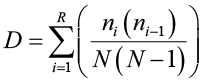 where ni is the number of individuals in species i, and N is the total number of species in the sample. An equivalent formula is:
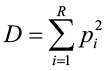 where pi is the proportional abundance for each species and R is the total number of species in the sample. Simpson’s index is a weighted arithmetic mean of proportional abundance and measures the probability that two individuals randomly selected from a sample will belong to the same species. Since the mean of the proportional abundance of the species increases with decreasing number of species and increasing abundance of the most abundant species, the value of D obtains small values in data sets of high diversity and large values in data sets with low diversity. The value of Simpson’s D ranges from 0 to 1, with 0 representing infinite diversity and 1 representing no diversity, so the larger the value of D, the lower the diversity. For this reason, Simpson’s index is usually expressed as its inverse (1/D) or its compliment (1-D) which is also known as the Gini-Simpson index.
Let’s look at an example. We want to compute Simpson’s D for this hypothetical community with three species.
Example 2
|
Species |
No. of individuals |
|
Sugar Maple |
35 |
|
Beech |
19 |
|
Yellow Birch |
11 |
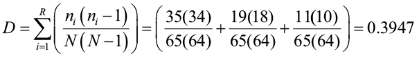
First, calculate N.
N = 35 + 19 + 11 = 65.
Then compute the index using the number of individuals for each species:
 The inverse is found to be:
1/0.3947 = 2.5336.
Using the inverse, the value of this index starts with 1 as the lowest possible figure. The higher the value of this inverse index the greater the diversity. If we use the compliment to Simpson’s D, the value is:
1-0.3947 = 0.6053.
This version of the index has values ranging from 0 to 1, but now, the greater the value, the greater the diversity of your sample. This compliment represents the probability that two individuals randomly selected from a sample will belong to different species. It is very important to clearly state which version of Simpson’s D you are using when comparing diversity.
Shannon-Weiner Index
The Shannon-Weiner index (Barnes et al. 1998) was developed from information theory and is based on measuring uncertainty. The degree of uncertainty of predicting the species of a random sample is related to the diversity of a community. If a community has low diversity (dominated by one species), the uncertainty of prediction is low; a randomly sampled species is most likely going to be the dominant species. However, if diversity is high, uncertainty is high. It is computed as:
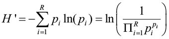
where pi is the proportion of individuals that belong to species i and R is the number of species in the sample. Since the sum of the pi’s equals unity by definition, the denominator equals the weighted geometric mean of the pi values, with the pi values being used as weights. The term in the parenthesis equals true diversity D and H’=ln(D). When all species in the data set are equally common, all pi values = 1/R and the Shannon-Weiner index equals ln(R). The more unequal the abundance of species, the larger the weighted geometric mean of the pi values, the smaller the index. If abundance is primarily concentrated into one species, the index will be close to zero.
An equivalent and computationally easier formula is:
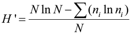
where N is the total number of species and ni is the number of individuals in species i. The Shannon-Weiner index is most sensitive to the number of species in a sample, so it is usually considered to be biased toward measuring species richness.
Let’s compute the Shannon-Weiner diversity index for the same hypothetical community in the previous example.
Example 2a
|
Species |
No. of individuals |
|
Sugar Maple |
35 |
|
Beech |
19 |
|
Yellow Birch |
11 |
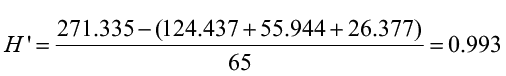
We know that N = 65. Now let’s compute the index:
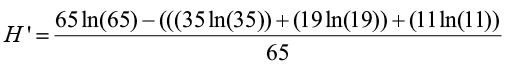 =
=
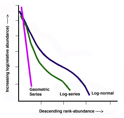
Rank Abundance Graphs
Species abundance distribution can also be expressed through rank abundance graphs. A common approach is to plot some measure of species abundance against their rank order of abundance. Such a plot allows the user to compare not only relative richness but also evenness. Species abundance models (also called abundance curves) use all available community information to create a mathematical model that describes the number and relative abundance of all species in a community. These models include the log normal, geometric, logarithmic, and MacArthur’s brokenstick model. Many ecologists use these models as a way to express resource partitioning where the abundance of a species is equivalent to the percentage of space it occupies (Magurran 1988). Abundance curves offer an alternative to single number diversity indices by graphically describing community structure.
Let’s compare the indices and a very simple abundance distribution in two different situations. Stand A and B both have the same number of species (same richness), but the number of individuals in each species is more similar in Stand A (greater evenness). In Stand B, species 1 has the most individuals, with the remaining nine species having a substantially smaller number of individuals per species. Richness, the compliment to Simpson’s D, and Shannon’s H’ are computed for both stands. These two diversity indices incorporate both richness and evenness. In the abundance distribution graph, richness can be compared on the x-axis and evenness by the shape of the distribution. Because Stand A displays greater evenness it has greater overall diversity than Stand B. Notice that Stand A has higher values for both Simpson’s and Shannon’s indices compared to Stand B.
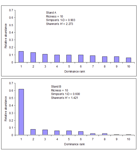
Indices of diversity vary in computation and interpretation so it is important to make sure you understand which index is being used to measure diversity. It is unsuitable to compare diversity between two areas when different indices are computed for each area. However, when multiple indices are computed for each area, the sampled areas will rank similarly in diversity as measured by the different indices. Notice in this previous example both Simpson’s and Shannon’s index rank Stand A as more diverse and Stand B as less diverse.
Similarity between Sites
There are also indices that compare the similarity (and dissimilarity) between sites. The ideal objective is to express the ecological similarity of different sites; however, it is important to identify the aim or focus of the investigation in order to select the most appropriate index. While many indices are available, van Tongeren (1995) states that most of the indices do not have a firm theoretical basis and suggests that practical experience should guide the selection of available indices.
The Jaccard index (1912) compares two sites based on the presence or absence of species and is used with qualitative data (e.g., species lists). It is based on the idea that the more species both sites have in common, the more similar they are. The Jaccard index is the proportion of species out of the total species list of the two sites, which is common to both sites:
SJ = c / (a + b + c)
where SJ is the similarity index, c is the number of shared species between the two sites and a and b are the number of species unique to each site. Sørenson (1948) developed a similarity index that is frequently referred to as the coefficient of community (CC):
CC = 2c / (a + b + 2c).
As you can see, this index differs from Jaccard’s in that the number of species shared between the two sites is divided by the average number of species instead of the total number of species for both sites. For both indices, the higher the value the more ecologically similar two sites are.
If quantitative data are available, a similarity ratio (Ball 1966) or a percentage similarity index, such as Gauch (1982), can be computed. Not only do these indices compare number of similar and dissimilar species present between two sites, but also incorporate abundance. The similarity ratio is:
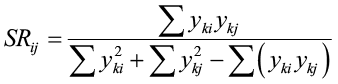
where yki is the abundance of the kth species at site i (sites i and j are compared). Notice that this equation resolves to Jaccard’s index when just presence or absence data is available. The percent similarity index is:
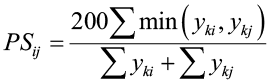
Again, notice how this equation resolves to Sørenson’s index with qualitative data only. So let’s look at a simple example of how these indices allow us to compare similarity between three sites. The following example presents hypothetical data on species abundance from three different sites containing seven different species (A-G).
Site |
|||
|
Species |
1 |
2 |
3 |
|
A |
4 |
0 |
1 |
|
B |
0 |
1 |
0 |
|
C |
0 |
0 |
0 |
|
D |
1 |
0 |
1 |
|
E |
1 |
4 |
0 |
|
F |
3 |
1 |
1 |
|
G |
1 |
0 |
3 |
Let’s begin by computing Jaccard’s and Sørenson’s indices for the three comparisons (site 1 vs. site 2, site 1 vs. site 3, and site 2 vs. site 3).
SJ1,2 =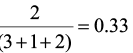 SJ1,3 =
 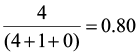 SJ2,3 =
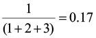
CC1,2 =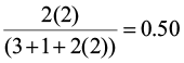 CC1,3 =
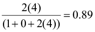 CC2,3 =
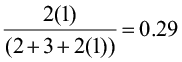
Both of these qualitative indices declare that sites 1 and 3 are the most similar and sites 2 and 3 are the least similar. Now let’s compute the similarity ratio and the percent similarity index for the same site comparisons.
SR1,2=
SR1,2= 0.23
SR1,3=
SR1,3= 0.38
SR2,3=
SR1,3= 0.03
PS1,2=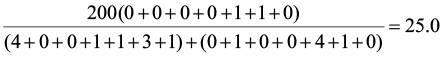
PS1,3=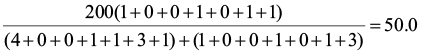
PS2,3=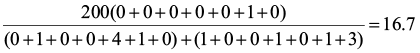
A matrix of percent similarity values allows for easy interpretation (especially when comparing more than three sites).

The quantitative indices return the same conclusions as the qualitative indices. Sites 1 and 3 are the most similar ecologically, and sites 2 and 3 are the least similar; and also site 2 is most unlike the other two sites.
Habitat Suitability Index (HSI)
In 1980, the U.S. Fish and Wildlife Service (USFWS) developed a procedure for documenting predicted impacts to fish and wildlife from proposed land and water resource development projects. The Habitat Evaluation Procedures (HEP) (Schamberger and Farmer 1978) were developed in response to the need to document the non-monetary value of fish and wildlife resources. HEP incorporates population and habitat theories for each species and is based on the assumption that habitat quality and quantity can be numerically described so that changes to the area could be assessed and compared. It is a species-habitat approach to impact assessment and habitat quality, for a specific species is quantified using a habitat suitability index (HSI).
Habitat suitability index (HSI) models provide a numerical index of habitat quality for a specific species (Schamberger et al. 1982) and in general assume a positive, linear relationship between carrying capacity (number of animals supported by some unit area) and HSI. Today’s natural resource manager often faces economically and socially important decisions that will affect not only timber but wildlife and its habitat. HSI models provide managers with tools to investigate the requirements necessary for survival of a species. Understanding the relationships between animal habitat and forest management prescription is vital towards a more comprehensive management approach of our natural resources. An HSI model synthesizes habitat use information into a framework appropriate for fieldwork and is scaled to produce an index value between 0.0 (unsuitable habitat) to 1.0 (optimum habitat), with each increment of change being identical to another. For example, a change in HSI from 0.4 to 0.5 represents the same magnitude of change as from 0.7 to 0.8. The HSI values are multiplied by area of available habitat to obtain Habitat Units (HUs) for individual species. The U.S. Fish and Wildlife Service (USFWS) has documented a series of HSI models for a wide variety of species (FWS/OBS-82/10).
Let’s examine a simple HSI model for the marten (Martes americana) which inhabits late successional forest communities in North America (Allen 1982). An HSI model must begin with habitat use information, understanding the species needs in terms of food, water, cover, reproduction, and range for this species. For this species, the winter cover requirements are more restrictive than cover requirements for any other season so it was assumed that if adequate winter cover was available, habitat requirements for the rest of the year would not be limiting. Additionally, all winter habitat requirements are satisfied in boreal evergreen forests. Given this, the research identified four crucial variables for winter cover that needed to be included in the model.
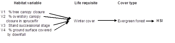
For each of these four winter cover variables (V1, V2, V3, and V4), suitability index graphs were created to examine the relationship between various conditions of these variables and suitable habitat for the marten. A reproduction of the graph for % tree canopy closure is presented below.
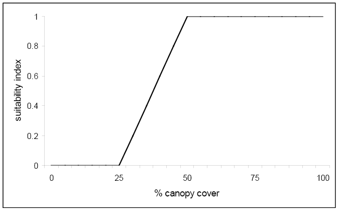
Notice that any canopy cover less than 25% results in unacceptable habitat based on this variable alone. However, once 50% canopy cover is reached the suitability index reaches 1.0 and optimum habitat for this variable is achieved. The following equation was created that combined the life requisite values for the marten using these four variables:
(V1 x V2 x V3 x V4) 1/2
Since winter cover was the only life requisite considered in this model, the HSI equals the winter cover value. As you can see, the more life requisites included in the model, the more complex the model becomes.
While HSI values identify the quality of the habitat for a specific species, wildlife diversity as a whole is a function of size and spatial arrangement of the treated stands (Porter 1986). Horizontal and structural diversity are important. Generally speaking, the more stands of different character an area contains, the greater the wildlife diversity. The spatial distribution of differing types of stands supports animals that need multiple cover types. In order to promote wildlife species diversity, a manager must develop forest management prescription that varies the spatial and temporal patterns of timber reproduction, thereby providing greater horizontal and vertical structural diversity.
Typically, even-aged management reduces vertical structural diversity, but options such as the shelterwood method tend to mitigate this problem. Selection system tends to promotes both horizontal and vertical diversity.
Integrated natural resource management can be a complicated process but not impossible. Vegetation response to silvicultural prescriptions provides the foundation for understanding the wildlife response. By examining the present characteristics of the managed stands, understanding the future response due to management, and comparing those with the requirements of specific species, we can achieve habitat manipulation together with timber management.
References
Aedrake09. “Modified logseries,” Wikipedia, http://en.wikipedia.org/wiki/File:Common_descriptiveWhittaker.jpg, 2009.
A.W. Allen, “Habitat Suitability Index Models: Marten,” U.S.D.I. Fish and Wildlife Service. FWS/OBS-82/10.11., 1982,9 pp.
B.V.Barnes et al., Forest Ecology 4th ed. , Wiley, 1998.
P. Jacard, “The Distribution of the Flora of the Alpine Zone,” New Phytologist 11, 1912, pp. 37-50.
A.E. Magurran, Ecological Diversity and Its Measurement, Princeton Univ. Press, 1988.
W.F. Porter, “Integrating Wildlife Management with Even-aged Timber Systems,” Managing Northern Hardwoods: Proceedings of a Silvicultural Symposium, ed. R. Nyland, SUNY College of Environmental Science and Forestry, 23-25 June, 1986, pp. 319-337.
M. Schamberger and A. Farmer, “The Habitat Evaluation Procedures: Their Application in Project Planning and Impact Evaluation,” Trans. N. A. Wildlife and Natural Resource Conf. 43, 1978, pp. 274-283.
E.H. Simpson, “Measurement of Diversity,” Nature 163, 1949, p. 688.
T. Sørenson, “A Method of Establishing Groups of Equal Amplitude in Plant Sociology Based on Similarity of Species Content,” Det. Kong. Danske Vidensk. Selsk. Biol. Skr. (Copenhagen) vol. 5, no. 4, 1948, pp. 1-34.
W.K. Strelke and J.G. Dickson, “Effect of Forest Clear-cut Edge on Breeding Birds in East Texas,” J. Wildl. Manage. vol, 44, no. 3, 1980, pp. 559-567.
U.S.D.I. Fish and Wildlife Service, “Habitat as a Basis for Environmental Assessment,” 101 ESM, 1980.
O.F.R. van Tongeren, “Cluster Analysis,” Data Analysis in Community and Landscape Ecology, Eds. R.H.G. Jongman, C.J.F. Ter Braak, and O.F.R. van Tongeren, 1995, pp. 174-212.
