Growth and Yield Models

Forest and natural resource management decisions are often based on information collected on past and present resource conditions. This information provides us with not only current details on the timber we manage (e.g., volume, diameter distribution) but also allows us to track changes in growth, mortality, and ingrowth over time. We use this information to make predictions of future growth and yield based on our management objectives. Techniques for forecasting stand dynamics are collectively referred to as growth and yield models. Growth and yield models are relationships between the amount of yield or growth and the many different factors that explain or predict this growth.

Before we continue our examination of growth and yield models, let’s review some basic terms.

Yield: total volume available for harvest at a given time

Growth: difference in volume between the beginning and end of a specified period of time (V2 – V1)

Annual growth: when growth is divided by number of years in the growing period

Model: a mathematical function used to relate observed growth rates or yield to measured tree, stand, and site variables

Estimation: a statistical process of obtaining coefficients for models that describe the growth rates or yield as a function of measured tree, stand, and site variables

Evaluation: considering how, where, and by whom the model should be used, how the model and its components operate, and the quality of the system design and its biological reality

Verification: the process of confirming that the model functions correctly with respect to the conceptual model. In other words, verification makes sure that there are no flaws in the programming logic or algorithms, and no bias in computation (systematic errors).

Validation: checks the accuracy and consistency of the model and tests the model to see how well it reflects the real system, if possible, using an independent data set

Simulation: using a computer program to simulate an abstract model of a particular system. We use a growth model to estimate stand development through time under alternative conditions or silvicultural practices.

Calibration: the process of modifying the model to account for local conditions that may differ from those on which the model was based

Monitoring: continually checking the simulation output of the system to identify any shortcomings of the model

Deterministic model: a model in which the outcomes are determined through known relationships among states and events, without any room for random variation. In forestry, a deterministic model provides an estimate of average stand growth, and given the same initial conditions, a deterministic model will always predict the same result.

Stochastic model: a model that attempts to illustrate the natural variation in a system by providing different predictions (each with a specific probability of occurrence) given the same initial conditions. A stochastic model requires multiple runs to provide estimates of the variability of predictions.

Process model: a model that attempts to simulate biological processes that convert carbon dioxide, nutrients, and moisture into biomass through photosynthesis

Succession model: a model that attempts to model species succession, but is generally unable to provide reliable information on timber yield

Models

Growth and yield models are typically stated as mathematical equations and can be implicit or explicit in form. An implicit model defines the variables in the equation but the specific relationship is not quantified. For example,

V = f (BA,Ht)

where V is volume (ft3/ac), BA is density (basal area in ft2), Ht is total tree height. This model says that volume is a function of (depends on) density and height, but it does not put a numerical value on the volume for specific values of basal area and height. This equation becomes explicit when we specify the relationship such as

ln(V) = -0.723 + 0.781*ln(BA)+ 0.922 ln(Ht)

Growth and yield models can be linear or nonlinear equations. In this linear model, all the independent variables of X1 and X2 are only raised to the first power.

y = 1.29 + 7.65 X1 -27.02 X2

A nonlinear model has independent variables with exponents different from one.

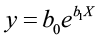
In this example, b0 and b1 are parameters to be estimated and X is the independent variable.

Classification of Growth and Yield Models

Growth and yield models have long been part of forestry but development and use has greatly increased in the last 25 years due to the accessibility of computers. There are many different approaches to modeling, each with their own advantages and disadvantages. Selecting a specific type of modeling approach often depends on the type of data used. Growth and yield models are categorized depending on whether they model the whole stand, the diameter classes, or individual trees.

Whole Stand Models

Whole stand models may or may not contain density as an independent variable. Density-free whole stand models provide the basis for traditional normal yield tables since “normal” implies nature’s maximum density, and empirical yield tables assume nature’s average density. In both of these cases, stand volume at a specific age is typically a function of stand age and site index. Variable-density whole stand models use density as an explicit independent variable to predict current or future volume. Buckman (1962) published the first study in the United States that directly predicted growth from current stand variables, then integrated the growth function to obtain yield:

Y = 1.6689 + 0.041066BA – 0.00016303BA2– 0.076958A + 0.00022741A2 + 0.06441S

where Y = periodic net annual basal area increment
BA = basal area, in square feet per acre
A = age, in years
S = site index

Diameter distribution models are a refinement of whole stand models. This type of model disaggregates the results at each age and then adds additional information about diameter class structure such as height and volume. The number of stems in each class is a function of the stand variables and all growth functions are for the stand. This type of whole stand model provides greater detail of the stand conditions in terms of volume, tree size, and value.

Diameter Class Models

Diameter class models (not to be confused with diameter distribution models) simulate growth and volume for each diameter class based on the average tree in each class. The number of trees in each class is empirically determined. The diameter class volumes are computed separately for each diameter class, then summed up to obtain stand values. Stand table projection is a common diameter class method used to predict short-term future conditions based on observable diameter growth for that stand. Mortality, harvest, and ingrowth must be computed separately. Differences in projection methods are based on the distribution of the number of stems in each class and how the growth rate is applied. For example, the simplest projection method is based on two assumptions: 1) that all tree diameters in a diameter class equal the midpoint diameter for that class, and 2) that they all grow at the same average rate. An improvement upon this method is to use a movement ratio that defines the proportion of trees which move into a higher DBH class.

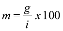
where m is the movement ratio, g is the average periodic diameter increment for that specific class, and i is the diameter class interval. Let’s look at an example.

Assume for a specific DBH class that g is 1.2 in. and i (class interval) is 2.0 in.

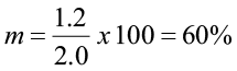
This means that 60% of the trees in that diameter class will move up to the next diameter class, and 40% will remain in this class. If the diameter class interval was one inch, the movement ratio would be different.

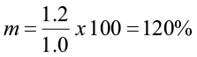
In this case, all the trees in this diameter class would move up at least one size class and 20% of them would move up two size classes.

Individual Tree Models

Individual tree models simulate the growth of each individual tree in the tree list. These models are more complex but have become more common as computing power has increased. Individual tree models typically simulate the height, diameter, and survival of each tree while calculating its growth. Individual tree data are aggregated after the model grows each tree, while stand models aggregate individual tree data into stand variables before the growth model is applied. Additionally, this type of model allows the user to include a measure of competition for each tree. Because of this, individual tree models are typically divided into two groups based on how competition is treated.

Distance-independent models define the competitive neighborhood for a subject tree by its own diameter, height, and condition to stand characteristics such as basal area, number of trees per area, and average diameter, however, the distances between trees are not required for computing the competition for each tree. Distance-dependent models include distance and bearing to all neighboring trees, along with their diameter. This way, the competitive neighborhood for each subject tree is precisely and uniquely defined. While this approach seems logically superior to distance-independent methods, there has not been any clear documented evidence to support the use of distance-dependent competition measures over distance-independent measures.

There are many growth and yield models and simulators available and it can be difficult to select the most appropriate model. There are advantages and disadvantages to many of these options and foresters must be concerned with the reliability of the estimates, the flexibility of the model to deal with management alternatives, the level of required detail, and the efficiency for providing information in a clear and useable fashion. Many models have been created using a broad range of available data. These models are best used for comparative purposes only. In other words, they are most appropriate when comparing the outcomes from different management options instead of predicting results for a specific stand. It is important to review and understand the foundations for any model or simulator before using it.

Forest Vegetation Simulator

The Forest Vegetation Simulator (FVS, Wykoff et al. 1982; Dixon 2002) is a distance-independent, individual-tree forest growth model commonly used in the United States to support forest management decisions. Projections are typically made at the stand level, but FVS has the ability to expand the spatial scope to much larger management units. FVS began as the Prognosis Model for Stand Development (Stage 1973) with the objective to predict stand dynamics in the mixed forests of Idaho and Montana. This model became the common modeling platform for the USDA Forest Service and was renamed FVS.

Stands are the basic unit of management and projections are dependent on the interactions among trees within stands using key variables such as density, species, diameter, height, crown ratio, diameter growth, and height growth. Values for slope, aspect, elevation, density, and a measure of site potential are included for each plot. There are 22 geographically specific versions of FVS called variants.

NE-TWIGS (Belcher 1982) is a common variant applicable to fourteen northeastern states. Stand growth projections are based on simulating the growth and mortality for trees in the 5-inch and larger DBH classes. Ingrowth can be manually entered or simulated using an automatic ingrowth function. The growth equation annually estimates a diameter for each sample tree and updates the crown ratio of the tree (Miner et al. 1988).

Annual diameter growth = potential growth*competition modifier

Potential growth is defined as the growth of the top 10% of the fastest growing trees and is predicted using the following equation:

where,

potential growth is defined as the potential annual basal area growth of a tree (sq. ft./yr)
b1 and b2 are species specific coefficients
SI is site index (index age 50 years) and
D is current tree diameter in in.

The competition modifier is an index bounded from 0 to 1, and is found by:

Competition modifier =

where b3 is a species-specific coefficient and
BA is the current basal area (sq. ft./ac).

Tree mortality is calculated by estimating the probability of death of each tree in a given year:

Survival = 1-[1/(1+en)]

where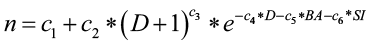
c1,…,c6 are species-specific coefficients
D is current tree diameter (inches)
BA is stand basal area (sq. ft./ac) and
SI is site index.

Inventory data and site information are entered into FVS, and a self-calibration process adjusts the growth models to match the rates present in the entered data. Harvests can be simulated with growth and mortality rates based on post-removal stand densities. Growth cycles run for 5-10 years and output includes a summary of current stand conditions, sampling statistics, and calibration results.

Applications of Regression Techniques

Regression models serve many purposes in the management of natural and forest resources. The following examples serve to highlight some of these applications.

Weight Scaling for Sawlogs

In 1962, Bower created the following equation for predicting loblolly pine sawlog volume based on truckload weights and the number of logs per truck:

Y = -3.954 N + 0.0925 W

where Y = total board-foot volume (International1/4- rule) for a truckload of logs
N = number of 16-ft logs on the truck
W = total load weight (lb.)

Notice that there is no y-intercept in the model. When there are no logs on the truck, there is no volume to be estimated.

Rates of Stem Taper

Kozak et al. (1969) developed a technique for estimating the fraction of volume per tree located in logs of any specified length and dib for any system of scaling (board feet, cubic feet, or weight). Their regression model also predicted taper curves and upper stem diameters (dib) for some conifer species.

where d = stem diameter at any height h above ground
H = total tree height

This equation resolves to:

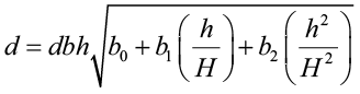
The predictor variables are the ratio, and squared ratio, of any height to total height.

Multiple Entry Volume Table that Allows for Variable Utilization Standards

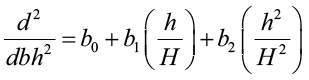
Foresters commonly want to predict tree volume for various top diameters but many of the available volume equations were created for specific top limits. Burkhart (1977) created a regression model to predict volume (cubic feet) of loblolly pine to any desired merchantable top limit. His approach predicted total stem volume, then converted total volume to merchantable volume by applying predicted ratios of merchantable volume to total volume.

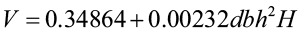
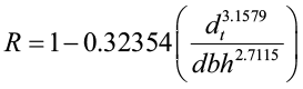
where dbh = diameter at breast height (in.)
H = total tree height (ft.)
V = total stem cubic-foot volume
R = merchantable cubic-foot volume to top diameter dt divided by total stem cubic-foot volume
dt = top dob (in.)

Weight Tables for Tree Boles

Belanger (1973) utilized a combined-variable approach to develop predictions of green-weight and dry weight of sycamore tree:

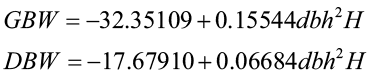
where GBW = green bole weight to 3-in.top (lb.)
DBW = dry bole weight to 3-in.top (lb.)
dbh = diameter at breast height (in.)
H = total tree height (ft.)

Biomass Prediction

A common approach to predicting tree biomass weight has been to use a logarithmic combined-variable formula (e.g. Edwards and McNab 1979). The observed relationship between these variables is typically non-linear, therefore a log or natural log transformation is needed to linearize the relationship.

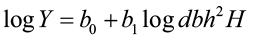
where Y = total tree weight
dbh = diameter at breast height
H = total tree height

However, past studies (Tritton and Hornbeck 1982 and Wiant et al. 1979) indicated that there was little model improvement when height was added. Many dry-weight biomass models now follow this form:

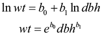
where wt = total tree weight
dbh = diameter at breast height

Volume Predictions based on Stump Diameter

Bylin (1982) created a regression model to predict tree volume using stump diameter and stump height for species in Louisiana.

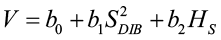
where V = tree volume (cu. ft.)
SDIB = stump diameters inside bark (in.)
HS = stump height (ft.)

Yield Estimation

MacKinney and Chaiken (1939) were the first to use multiple regression, with stand density as a predictor variable, to predict yield for loblolly pine trees.

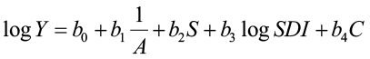
where Y = yield (cu. ft./ac)
A = stand age
S = site index
SDI = stand-density index
C = composition index (loblolly pine BA/total BA)

Growth and Yield Prediction for Uneven-aged Stands

Moser and Hall (1969) developed a yield equation, expressed as a function of time, initial volume, and basal area, to predict volume in mixed northern hardwoods.

where Y0 = initial volume (cu. ft./ac)
BA0 = initial basal area (sq. ft./ac)
t = elapsed time interval (years from initial condition)
Y = predicted volume (cu. ft./ac) t years after observation of initial conditions Y0 and BA0 at time t0

Site Index

Site is defined by the Society of American Foresters (1971) as “an area considered in terms of its own environment, particularly as this determines the type and quality of the vegetation the area can carry.” Forest and natural resource managers use site measurement to identify the potential productivity of a forest stand and to provide a comparative frame of reference for management options. The productive potential or capacity of a site is often referred to as site quality.

Site quality can be measured directly or indirectly. Direct measurement of a stand’s productivity can be measured by analyzing the variables such as soil nutrients, moisture, temperature regimes, available light, slope, and aspect. A productivity-estimation method based on the permanent features of soil and topography can be used on any site and is suitable in areas where forest stands do not presently exist. Soil site index is an example of such an index. However, such indices are location specific and should not be used outside the geographic region in which they were developed. Unfortunately, environmental factor information is not always available and natural resource managers must use alternative methods.

Historical yield records also provide direct evidence of a site’s productivity by averaging the yields over multiple rotations or cutting cycles. Unfortunately, there are limited long-term data available, and yields may be affected by species composition, stand density, pests, rotation age, and genetics. Consequently, indirect methods of measuring site quality are frequently used, with the most common involving the relationship between tree height and tree age.

Using stand height data is an easy and reliable way to quantify site quality. Theoretically, height growth is sensitive to differences in site quality and height development of larger trees in an even-aged stand is seldom affected by stand density. Additionally, the volume-production potential is strongly correlated with height-growth rate. This measure of site quality is called site index and is the average total height of selected dominant-codominant trees on a site at a particular reference or index age. If you measure a stand that is at an index age, the average height of the dominant and codominant trees is the site index. It is the most widely accepted quantitative measure of site quality in the United States for even-aged stands (Avery and Burkhart 1994).

The objective of the site index method is to select the height development pattern that the stand can be expected to follow during the remainder of its life (not to predict stand height at the index age). Most height-based methods of site quality evaluation use site index curves. Site index curves are a family of height development patterns referenced by either age at breast height or total age. For example, site index curves for plantations are generally based on total age (years since planted), where age at breast height is frequently used for natural stands for the sake of convenience. If total age were to be used in this situation, the number of years required for a tree to grow from a seedling to DBH must be added in. Site index curves can either be anamorphic or polymorphic curves. Anamorphic curves (most common) are a family of curves with the same shape but different intercepts. Polymorphic curves are a family of curves with different shapes and intercepts.

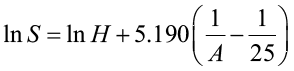
The index age for this method is typically the culmination of mean annual growth. In the western part of the United States, 100 years is commonly used as the reference age with 50 years in the eastern part of this country. However, site index curves can be based on any index age that is needed. Coile and Schumacher (1964) created a family of anamorphic site index curves for plantation loblolly pine with an index age of 25 years. The following family of anamorphic site index curves for a southern pine is based on a reference age of 50 years.

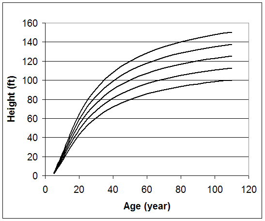
Creating a site index curve involves the random selection of dominant and codominant trees, measuring their total height, and statistically fitting the data to a mathematical equation. So, which equation do you use? Plotting height over age for single species, even-aged stands typically results in a sigmoid shaped pattern.

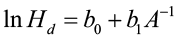
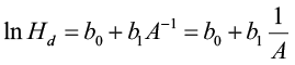
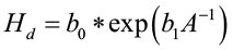where Hd is the height of dominant and codominant trees, A is stand age, and b0 and b1 are coefficients to be estimated. Variable transformation is needed if linear regression is to be used to fit the model. A common transformation is

Coile and Schumacher (1964) fit their data to the following model:

where S is site index, H is total tree height, and A is average age. The site index curve is created by fitting the model to data from stands of varying site qualities and ages, making sure that all necessary site index classes are equally represented at all ages. It is important not to bias the curve by using an incomplete range of data.

Data for the development of site index equations can come from measurement of tree or stand height and age from temporary or permanent inventory plots or from stem analysis. Inventory plot data are typically used for anamorphic curves only and sampling bias can occur when poor sites are over represented in older age classes. Stem analysis can be used for polymorphic curves but requires destructive sampling and it can be expensive to obtain such data.

We are going to examine three different methods for developing site index equations:

1. Guide curve method
2. Difference equation method
3. Parameter prediction method

Guide Curve Method

The guide curve method is commonly used to generate anamorphic site index equations. Let’s begin with a commonly used model form:

 [1]

Parameterizing this model results in a “guide curve” (the average line for the sample data) that is used to create the individual height/age development curves that parallel the guide curve. For a particular site index the equation is:

[2]

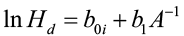
where boi is the unique y-intercept for that age. By definition, when A = A0 (index age), H is equal to site index S. Thus:

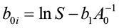[3]

Substituting boi into equation [2] gives:

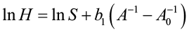[4]

which can be used to generate site index curves for given values of S and A0 and a range of ages (A). The equation can be algebraically rearranged as:

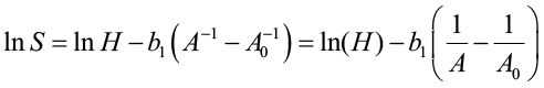[5]

This is the form to estimate site index (height at index age) when height and age data measurements are given. This process is sound only if the average site quality in the sample data is approximately the same for all age classes. If the average site quality varies systematically with age, the guide curve will be biased.

Difference Equation Method

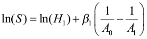
This method requires either monumented plot, tree remeasurement data, or stem analysis data. The model is fit using differences of height and specific ages. This method is appropriate for anamorphic and polymorphic curves, especially for longer and/or multiple measurement periods. Schumacher (after Clutter et al. 1983) used this approach when estimating site index using the reciprocal of age and the natural log of height. He believed that there was a linear relationship between Point A (1/A1, lnH1) and Point B (1/A2, lnH2) and defined β1 (slope) as:

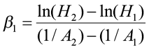
where H1 and A1 were initial height and age, and H2 and A2 were height and age at the end of the remeasurement period. His height/age model became:

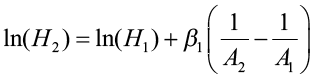
Using remeasurement data, this equation would be fitted using linear regression procedures with the model

where Y = ln(H2) – ln(H1)
X = (1/A2) – (1/A1)

After estimating β1, a site index equation is obtained from the height/age equation by letting A2 equal A0 (the index age) so that H2 is, by definition, site index (S). The equation can then be written:

Parameter Prediction Method

This method requires remeasurement or stem analysis data, and involves the following steps:

1. Fitting a linear or nonlinear height/age function to the data on a tree-by-tree (stem analysis data) or plot by plot (remeasurement data) basis
2. Using each fitted curve to assign a site index value to each tree or plot (put A0 in the equation to estimate site index)
3. Relating the parameters of the fitted curves to site index through linear or nonlinear regression procedures

Trousdell et al. (1974) used this approach to estimate site index for loblolly pine and it provides an example using the Chapman-Richards (Richards 1959) function for the height/age relationship. They collected stem analysis data on 44 dominant and codominant trees that had a minimum age of at least 50 years. The Chapman-Richards function was used to define the height/age relationship:

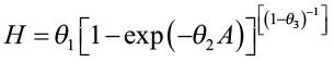
where H is height in feet at age A and θ1, θ2, and θ3 are parameters to be estimated. This equation was fitted separately to each tree. The fitted curves were all solved with A = 50 to obtain site index values (S) for each tree.

The parameters θ1, θ2, and θ3 were hypothesized to be functions of site index, where

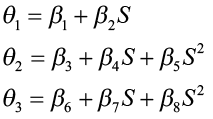
The Chapman-Richards function was then expressed as:

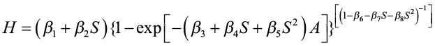
This function was then refitted to the data to estimate the parameters β1, β2, …β8. The estimating equations obtained for θ1, θ2, and θ3 were

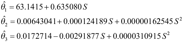
For any given site index value, these equations can be solved to give a particular Chapman-Richards site index curve. By substituting various values of age into the equation and solving for H, we obtain height/age points that can be plotted for a site index curve. Since each site index curve has different parameter values, the curves are polymorphic.

Periodic Height Growth Data

An alternative to using current stand height as the surrogate for site quality is to use periodic height growth data, which is referred to as a growth intercept method. This method is practical only for species that display distinct annual branch whorls and is primarily used for juvenile stands because site index curves are less dependable for young stands.

This method requires the length measurement of a specified number of successive annual internodes or the length over a 5-year period. While the growth-intercept values can be used directly as measures of site quality, they are more commonly used to estimate site index.

Alban (1972) created a simple linear model to predict site index for red pine using 5-year growth intercept in feet beginning at 8 ft. above ground.

SI = 32.54 + 3.43 X

where SI is site index at a base age of 50 years and X is 5-year growth intercept in feet.

Using periodic height growth data has the advantage of not requiring stand age or total tree height measurements, which can be difficult in young, dense stands. However, due to the short-term nature of the data, weather variation may strongly influence the internodal growth thereby rendering the results inaccurate.

Site index equations should be based on biological or mathematical theories, which will help the equation perform better. They should behave logically and not allow unreasonable values for predicted height, especially at very young or very old ages. The equations should also contain an asymptotic parameter to control unbounded height growth at old age. The asymptote should be some function of site index such that the asymptote increases with increases of site index.

When using site index, it is important to know the base age for the curve before use. It is also important to realize that site index based on one base age cannot be converted to another base age. Additionally, similar site indices for different species do not mean similar sites even when the same base age is used for both species. You have to understand how height and age were measured before you can safely interpret a site index curve. Site index is not a true measure of site quality; rather it is a measure of a tree growth component that is affected by site quality (top height is a measure of stand development, NOT site quality).

References

D.H. Alban, “An Improved Growth Intercept Method for Estimating Site Index of Red Pine,” U.S. Forest Serv., North Central Forest Expt. Sta., Res. Paper NC-80, 1972, p. 7.

T.E. Avery and H.E. Burkhart, Forest Measurements,. McGraw-Hill, 1994, p. 408.

R.P. Belanger, “Volume and Weight Tables for Plantation-grown Sycamore,” U.S. Forest Serv. Southeast. Forest Expt. Sta. Res. Paper SE-107, 1973, p. 8.

D.M. Belcher, “TWIGS: The Woodman’s Ideal Growth Projection System,” Microcomputers, a New Tool for Foresters, Purdue University Press, 1982, p. 70.

D.R. Bower, “Volume-weight Relationships for Loblolly Pine Sawlogs,” J. Forestry 60, 1962, pp. 411-412.

R.R. Buckman, “Growth and Yield of Red Pine in Minnesota,” U.S. Department of Agriculture, Technical Bulletin 1272, 1962.

H.E. Burkhart, “Cubic-foot Volume of Loblolly Pine to Any Merchantable Top Limit,” So. J. Appl. For. 1, 1977, pp. 7-9.

C.V. Bylin, “Volume Prediction from Stump Diameter and Stump Height of Selected Species in Louisiana,” U.S. Forest Serv., Southern Forest. Expt. Sta., Res. Paper SO-182, 1982, p. 11.

J.R. Clutter Et al., Timber Management: A Quantitative Approach, Wiley, 1983, p. 333.

T.S. Coile and F. X. Schumacher, Soil-site Relations, Stand Structure, and Yields of Slash and Loblolly Pine Plantations in the Southern United States, T.S. Coile, 1964.

G.E. Dixon (Comp.), “Essential FVS: A User’s Guide to the Forest Vegetation Simulator,” Internal Report. U.S. Department of Agriculture, Forest Service, Forest Management Service Center, 2002, p. 189.

M.B. Edwards and W.H. McNab, “Biomass Prediction for Young Southern Pines,” J. Forestry, 77, 1979, pp. 291-292.

A.D. Kozak, D.D. Munro, and J.H.G. Smith, “Taper Functions and Their Application in Forest Inventory,” Forestry Chronicle 45, 1969, pp. 278-283.

A.L. MacKinney and L.E. Chaiken, “Volume, Yield, and Growth of Loblolly Pine in the Mid-Atlantic Coastal Region,” U.S. Forest. Serv. Appalachian Forest Expt. Sta., Tech. Note 33, 1939, p. 30.

C.L. Miner, N.R. Walters, and M.L. Belli, “A Guide to the TWIGS Program for the North Central United States,” USDA Forest Serv., North Central Forest Exp.Sta., Gen. Tech. Rep. NC-125, 1988, p. 105.

J.W. Moser, Jr. and O.F. Hall, “Deriving Growth and Yield Functions for Uneven-aged Forest Stands,” Forest Sci. 15, 1969, pp. 183-188.

F.J. Richards, “A Flexible Growth Function for Empirical Use,” J. Exp. Botany, vol. 10, no. 2 1959, pp. 290-300.

Society of American Foresters, Terminology of Forest Science, Technology, Practice, and Products, Washington,D.C., Society of American Foresters, 1971, p. 349.

A.R. Stage, “Prognosis Model for Stand Development,” U.S. Department of Agriculture, Forest Service, Intermountain Forest and Range Expt. Sta., Res. Pa INT-137, 1973, p. 32.

L.M. Tritton and J.W. Hornbeck, “Biomass Equations for Major Tree Species of the Northeast,” USDA For. Serv. Gen. Tech. Rep. NE-GTR-69, 1982.

K.B. Trousdell, D.E. Beck, and F.T. Lloyd, “Site Index for Loblolly Pine in the Atlantic Coastal Plain of the Carolinas and Virginia,” U.S. Southeastern Forest Expt. Sta., 1974, p. 115.

H.J. Wiant et al., “Equations for Predicting Weights of Some Appalachian Hardwoods,” West Virginia Univ. Agric. and Forest Expt. Sta., Coll.. of Agric. and Forest. West Virginia Forest. Notes, no. 7, 1979.

W.R. Wykoff, N.L. Crookston, and A.R. Stage, “User’s Guide to the Stand Prognosis Model,” U.S. Department of Agriculture, Forest Service, Intermountain Forest and Range Expt. Sta., Gen. Tech. Re INT-133, 1982, p. 112.