
Chapter 6: Two-way Analysis of Variance
In the previous chapter we used one-way ANOVA to analyze data from three or more populations using the null hypothesis that all means were the same (no treatment effect). For example, a biologist wants to compare mean growth for three different levels of fertilizer. A one-way ANOVA tests to see if at least one of the treatment means is significantly different from the others. If the null hypothesis is rejected, a multiple comparison method, such as Tukey’s, can be used to identify which means are different, and the confidence interval can be used to estimate the difference between the different means.
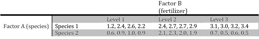
Suppose the biologist wants to ask this same question but with two different species of plants while still testing the three different levels of fertilizer. The biologist needs to investigate not only the average growth between the two species (main effect A) and the average growth for the three levels of fertilizer (main effect B), but also the interaction or relationship between the two factors of species and fertilizer. Two-way analysis of variance allows the biologist to answer the question about growth affected by species and levels of fertilizer, and to account for the variation due to both factors simultaneously.
Our examination of one-way ANOVA was done in the context of a completely randomized design where the treatments are assigned randomly to each subject (or experimental unit). We now consider analysis in which two factors can explain variability in the response variable. Remember that we can deal with factors by controlling them, by fixing them at specific levels, and randomly applying the treatments so the effect of uncontrolled variables on the response variable is minimized. With two factors, we need a factorial experiment.
This is an example of a factorial experiment in which there are a total of 2 x 3 = 6 possible combinations of the levels for the two different factors (species and level of fertilizer). These six combinations are referred to as treatments and the experiment is called a 2 x 3 factorial experiment. We use this type of experiment to investigate the effect of multiple factors on a response and the interaction between the factors. Each of the n observations of the response variable for the different levels of the factors exists within a cell. In this example, there are six cells and each cell corresponds to a specific treatment.
When you compare treatment means for a factorial experiment (or for any other experiment), multiple observations are required for each treatment. These are called replicates. For example, if you have four observations for each of the six treatments, you have four replications of the experiment. Replication demonstrates the results to be reproducible and provides the means to estimate experimental error variance. Replication also provides the capacity to increase the precision for estimates of treatment means. Increasing replication decreases  =
=  thereby increasing the precision of
|
Notation |
|
k = number of levels of factor A |
|
l = number of levels of factor B |
|
kl = number of treatments (each one a combination of a factor A level and a factor B level) |
|
m = number of observations on each treatment |
Main Effects and Interaction Effect
Main effects deal with each factor separately. In the previous example we have two factors, A and B. The main effect of Factor A (species) is the difference between the mean growth for Species 1 and Species 2, averaged across the three levels of fertilizer. The main effect of Factor B (fertilizer) is the difference in mean growth for levels 1, 2, and 3 averaged across the two species. The interaction is the simultaneous changes in the levels of both factors. If the changes in the level of Factor A result in different changes in the value of the response variable for the different levels of Factor B, we say that there is an interaction effect between the factors. Consider the following example to help clarify this idea of interaction.
Example 1
Factor A has two levels and Factor B has two levels. In the left box, when Factor A is at level 1, Factor B changes by 3 units. When Factor A is at level 2, Factor B again changes by 3 units. Similarly, when Factor B is at level 1, Factor A changes by 2 units. When Factor B is at level 2, Factor A again changes by 2 units. There is no interaction. The change in the true average response when the level of either factor changes from 1 to 2 is the same for each level of the other factor. In this case, changes in levels of the two factors affect the true average response separately, or in an additive manner.
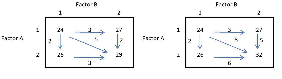
The right box illustrates the idea of interaction. When Factor A is at level 1, Factor B changes by 3 units but when Factor A is at level 2, Factor B changes by 6 units. When Factor B is at level 1, Factor A changes by 2 units but when Factor B is at level 2, Factor A changes by 5 units. The change in the true average response when the levels of both factors change simultaneously from level 1 to level 2 is 8 units, which is much larger than the separate changes suggest. In this case, there is an interaction between the two factors, so the effect of simultaneous changes cannot be determined from the individual effects of the separate changes. Change in the true average response when the level of one factor changes depends on the level of the other factor. You cannot determine the separate effect of Factor A or Factor B on the response because of the interaction.
Assumptions
Basic Assumption: The observations on any particular treatment are independently selected from a normal distribution with variance σ2 (the same variance for each treatment), and samples from different treatments are independent of one another.
We can use normal probability plots to satisfy the assumption of normality for each treatment. The requirement for equal variances is more difficult to confirm, but we can generally check by making sure that the largest sample standard deviation is no more than twice the smallest sample standard deviation.
Although not a requirement for two-way ANOVA, having an equal number of observations in each treatment, referred to as a balance design, increases the power of the test. However, unequal replications (an unbalanced design), are very common. Some statistical software packages (such as Excel) will only work with balanced designs. Minitab will provide the correct analysis for both balanced and unbalanced designs in the General Linear Model component under ANOVA statistical analysis. However, for the sake of simplicity, we will focus on balanced designs in this chapter.
Sums of Squares and the ANOVA Table
In the previous chapter, the idea of sums of squares was introduced to partition the variation due to treatment and random variation. The relationship is as follows:
SSTo = SSTr + SSE
We now partition the variation even more to reflect the main effects (Factor A and Factor B) and the interaction term:
SSTo = SSA + SSB +SSAB +SSE
where
- SSTo is the total sums of squares, with the associated degrees of freedom klm – 1
- SSA is the factor A main effect sums of squares, with associated degrees of freedom k – 1
- SSB is the factor B main effect sums of squares, with associated degrees of freedom l – 1
- SSAB is the interaction sum of squares, with associated degrees of freedom (k – 1)(l – 1)
- SSE is the error sum of squares, with associated degrees of freedom kl(m – 1)
As we saw in the previous chapter, the magnitude of the SSE is related entirely to the amount of underlying variability in the distributions being sampled. It has nothing to do with values of the various true average responses. SSAB reflects in part underlying variability, but its value is also affected by whether or not there is an interaction between the factors; the greater the interaction, the greater the value of SSAB.
The following ANOVA table illustrates the relationship between the sums of squares for each component and the resulting F-statistic for testing the three null and alternative hypotheses for a two-way ANOVA.
- H0: There is no interaction between factors
H1: There is a significant interaction between factors - H0: There is no effect of Factor A on the response variable
H1: There is an effect of Factor A on the response variable - H0: There is no effect of Factor B on the response variable
H1: There is an effect of Factor B on the response variable
If there is a significant interaction, then ignore the following two sets of hypotheses for the main effects. A significant interaction tells you that the change in the true average response for a level of Factor A depends on the level of Factor B. The effect of simultaneous changes cannot be determined by examining the main effects separately. If there is NOT a significant interaction, then proceed to test the main effects. The Factor A sums of squares will reflect random variation and any differences between the true average responses for different levels of Factor A. Similarly, Factor B sums of squares will reflect random variation and the true average responses for the different levels of Factor B.
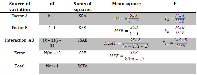
Each of the five sources of variation, when divided by the appropriate degrees of freedom (df), provides an estimate of the variation in the experiment. The estimates are called mean squares and are displayed along with their respective sums of squares and df in the analysis of variance table. In one-way ANOVA, the mean square error (MSE) is the best estimate of σ2 (the population variance) and is the denominator in the F-statistic. In a two-way ANOVA, it is still the best estimate of σ2. Notice that in each case, the MSE is the denominator in the test statistic and the numerator is the mean sum of squares for each main factor and interaction term. The F-statistic is found in the final column of this table and is used to answer the three alternative hypotheses. Typically, the p-values associated with each F-statistic are also presented in an ANOVA table. You will use the Decision Rule to determine the outcome for each of the three pairs of hypotheses.
If the p-value is smaller than α (level of significance), you will reject the null hypothesis.
When we conduct a two-way ANOVA, we always first test the hypothesis regarding the interaction effect. If the null hypothesis of no interaction is rejected, we do NOT interpret the results of the hypotheses involving the main effects. If the interaction term is NOT significant, then we examine the two main effects separately. Let’s look at an example.
Example 2
An experiment was carried out to assess the effects of soy plant variety (factor A, with k = 3 levels) and planting density (factor B, with l = 4 levels – 5, 10, 15, and 20 thousand plants per hectare) on yield. Each of the 12 treatments (k * l) was randomly applied to m = 3 plots (klm = 36 total observations). Use a two-way ANOVA to assess the effects at a 5% level of significance.
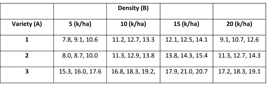
It is always important to look at the sample average yields for each treatment, each level of factor A, and each level of factor B.
|
Density |
|||||
|
Variety |
5 |
10 |
15 |
20 |
Sample average yield for each level of factor A |
|
1 |
9.17 |
12.40 |
12.90 |
10.80 |
11.32 |
|
2 |
8.90 |
12.67 |
14.50 |
12.77 |
12.21 |
|
3 |
16.30 |
18.10 |
19.87 |
18.20 |
18.12 |
|
Sample average yield for each level of factor B |
11.46 |
14.39 |
15.77 |
13.92 |
13.88 |
Table 4. Summary table.
For example, 11.32 is the average yield for variety #1 over all levels of planting densities. The value 11.46 is the average yield for plots planted with 5,000 plants across all varieties. The grand mean is 13.88. The ANOVA table is presented next.
|
Source |
DF |
SS |
MSS |
F |
P |
|
variety |
2 |
327.774 |
163.887 |
100.48 |
<0.001 |
|
density |
3 |
86.908 |
28.969 |
17.76 |
<0.001 |
|
variety*density |
6 |
8.068 |
1.345 |
0.82 |
0.562 |
|
error |
24 |
39.147 |
1.631 |
||
|
total |
35 |
Table 5. Two-way ANOVA table.
You begin with the following null and alternative hypotheses:
H0: There is no interaction between factors
H1: There is a significant interaction between factors
The F-statistic: 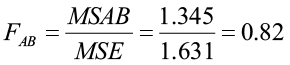
The p-value for the test for a significant interaction between factors is 0.562. This p-value is greater than 5% (α), therefore we fail to reject the null hypothesis. There is no evidence of a significant interaction between variety and density. So it is appropriate to carry out further tests concerning the presence of the main effects.
H0: There is no effect of Factor A (variety) on the response variable
H1: There is an effect of Factor A on the response variable
The F-statistic: 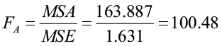
The p-value (<0.001) is less than 0.05 so we will reject the null hypothesis. There is a significant difference in yield between the three varieties.
H0: There is no effect of Factor B (density) on the response variable
H1: There is an effect of Factor B on the response variable
The F-statistic: 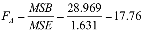
The p-value (<0.001) is less than 0.05 so we will reject the null hypothesis. There is a significant difference in yield between the four planting densities.
Multiple Comparisons
The next step is to examine the multiple comparisons for each main effect to determine the differences. We will proceed as we did with one-way ANOVA multiple comparisons by examining the Tukey’s Grouping for each main effect. For factor A, variety, the sample means, and grouping letters are presented to identify those varieties that are significantly different from other varieties. Varieties 1 and 2 are not significantly different from each other, both producing similar yields. Variety 3 produced significantly greater yields than both variety 1 and 2.
|
Grouping Information Using Tukey Method and 95.0% Confidence |
||||
|
variety |
N |
Mean |
Grouping |
|
|
3 |
12 |
18.117 |
A |
|
|
2 |
12 |
12.208 |
B |
|
|
1 |
12 |
11.317 |
B |
|
|
Means that do not share a letter are significantly different. |
||||
Some of the densities are also significantly different. We will follow the same procedure to determine the differences.
|
Grouping Information Using Tukey Method and 95.0% Confidence |
|||||
|
density |
N |
Mean |
Grouping |
||
|
15 |
9 |
15.756 |
A |
||
|
10 |
9 |
14.389 |
A |
B |
|
|
20 |
9 |
13.922 |
B |
||
|
5 |
9 |
11.456 |
C |
||
|
Means that do not share a letter are significantly different. |
|||||
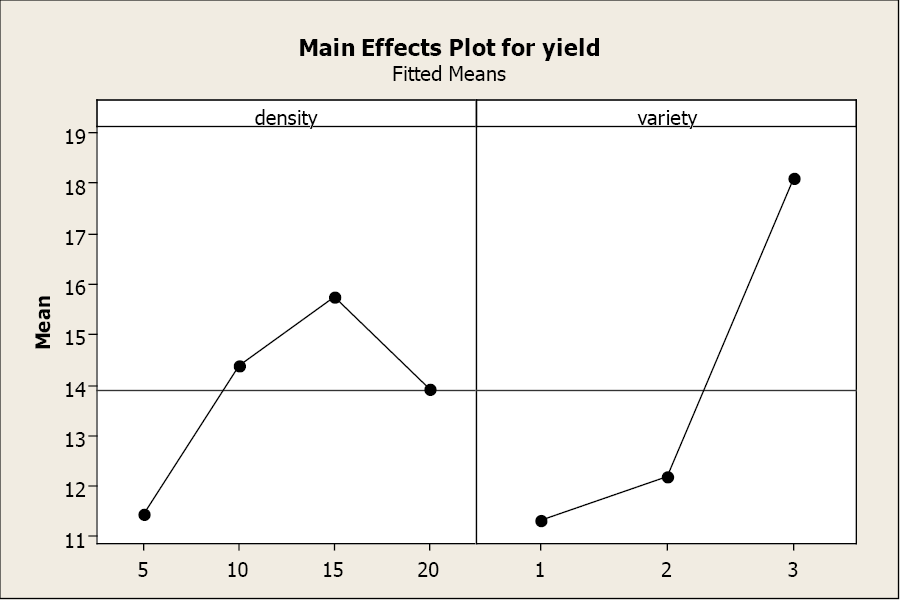
The Grouping Information shows us that a planting density of 15,000 plants/plot results in the greatest yield. However, there is no significant difference in yield between 10,000 and 15,000 plants/plot or between 10,000 and 20,000 plants/plot. The plots with 5,000 plants/plot result in the lowest yields and these yields are significantly lower than all other densities tested.
The main effects plots also illustrate the differences in yield across the three varieties and four densities.
But what happens if there is a significant interaction between the main effects? This next example will demonstrate how a significant interaction alters the interpretation of a 2-way ANOVA.
Example 3
A researcher was interested in the effects of four levels of fertilization (control, 100 lb., 150 lb., and 200 lb.) and four levels of irrigation (A, B, C, and D) on biomass yield. The sixteen possible treatment combinations were randomly assigned to 80 plots (5 plots for each treatment). The total biomass yields for each treatment are listed below.
|
Fertilizer |
||||
|
Irrigation |
Control |
100 lb. |
150 lb. |
200 lb. |
|
A |
2700,2801,2720, 2390, 2890 |
3250, 3151, 3170, 3300, 3290 |
3300, 3235, 3025, 3165, 3120 |
3500, 3455, 3100, 3600, 3250 |
|
B |
3101, 3035, 3205, 3007, 3100 |
2700, 2935, 2250, 2495, 2850 |
3050, 3110, 3033, 3195, 4250 |
3100, 3235, 3005, 3095, 3050 |
|
C |
101, 97, 106, 142, 99 |
400, 302, 296, 315, 390 |
630, 624, 595, 675, 595 |
400, 325, 200, 375, 390 |
|
D |
121, 174, 88, 100, 76 |
100, 125, 91, 222, 219 |
60, 28, 112, 89, 67 |
201, 223, 195, 120, 180 |
Table 6. Observed data for four irrigation levels and four fertilizer levels.
Factor A (irrigation level) has k = 4 levels and factor B (fertilizer) has l = 4 levels. There are m = 5 replicates and 80 total observations. This is a balanced design as the number of replicates is equal. The ANOVA table is presented next.
|
Source |
DF |
SS |
MSS |
F |
P |
|
fertilizer |
3 |
1128272 |
376091 |
12.76 |
<0.001 |
|
irrigation |
3 |
161776127 |
53925376 |
1830.16 |
<0.001 |
|
fert*irrigation |
9 |
2088667 |
232074 |
7.88 |
<0.001 |
|
error |
64 |
1885746 |
29465 |
||
|
total |
79 |
166878812 |
Table 7. Two-way ANOVA table.
We again begin with testing the interaction term. Remember, if the interaction term is significant, we ignore the main effects.
H0: There is no interaction between factors
H1: There is a significant interaction between factors
The F-statistic: 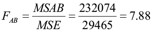
The p-value for the test for a significant interaction between factors is <0.001. This p-value is less than 5%, therefore we reject the null hypothesis. There is evidence of a significant interaction between fertilizer and irrigation. Since the interaction term is significant, we do not investigate the presence of the main effects. We must now examine multiple comparisons for all 16 treatments (each combination of fertilizer and irrigation level) to determine the differences in yield, aided by the factor plot.
|
Grouping Information Using Tukey Method and 95.0% Confidence |
|||||||
|
fert |
irrigation |
N |
Mean |
Grouping |
|||
|
200 |
A |
5 |
3381.00 |
A |
|||
|
150 |
B |
5 |
3327.60 |
A |
|||
|
100 |
A |
5 |
3232.20 |
A |
|||
|
150 |
A |
5 |
3169.00 |
A |
|||
|
200 |
B |
5 |
3097.00 |
A |
|||
|
C |
B |
5 |
3089.60 |
A |
|||
|
C |
A |
5 |
2700.20 |
B |
|||
|
100 |
B |
5 |
2646.00 |
B |
|||
|
150 |
C |
5 |
623.80 |
C |
|||
|
100 |
C |
5 |
340.60 |
C |
D |
||
|
200 |
C |
5 |
338.00 |
C |
D |
||
|
200 |
D |
5 |
183.80 |
D |
|||
|
100 |
D |
5 |
151.40 |
D |
|||
|
C |
D |
5 |
111.80 |
D |
|||
|
C |
C |
5 |
109.00 |
D |
|||
|
150 |
D |
5 |
71.20 |
D |
|||
|
Means that do not share a letter are significantly different. |
|||||||
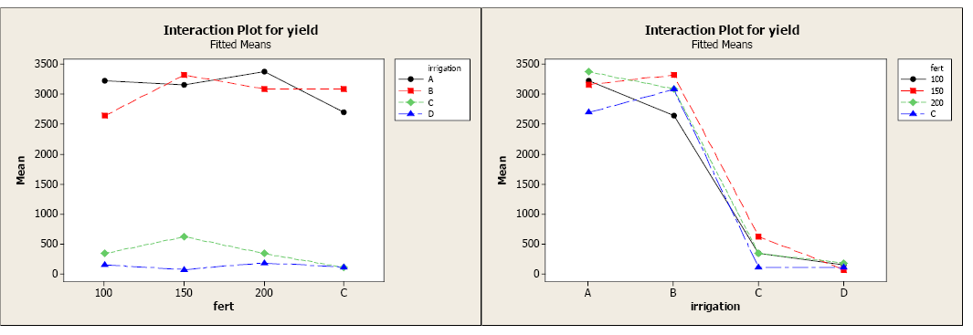
The factor plot allows you to visualize the differences between the 16 treatments. Factor plots can present the information two ways, each with a different factor on the x-axis. In the first plot, fertilizer level is on the x-axis. There is a clear distinction in average yields for the different treatments. Irrigation levels A and B appear to be producing greater yields across all levels of fertilizers compared to irrigation levels C and D. In the second plot, irrigation level is on the x-axis. All levels of fertilizer seem to result in greater yields for irrigation levels A and B compared to C and D.
The next step is to use the multiple comparison output to determine where there are SIGNIFICANT differences. Let’s focus on the first factor plot to do this.
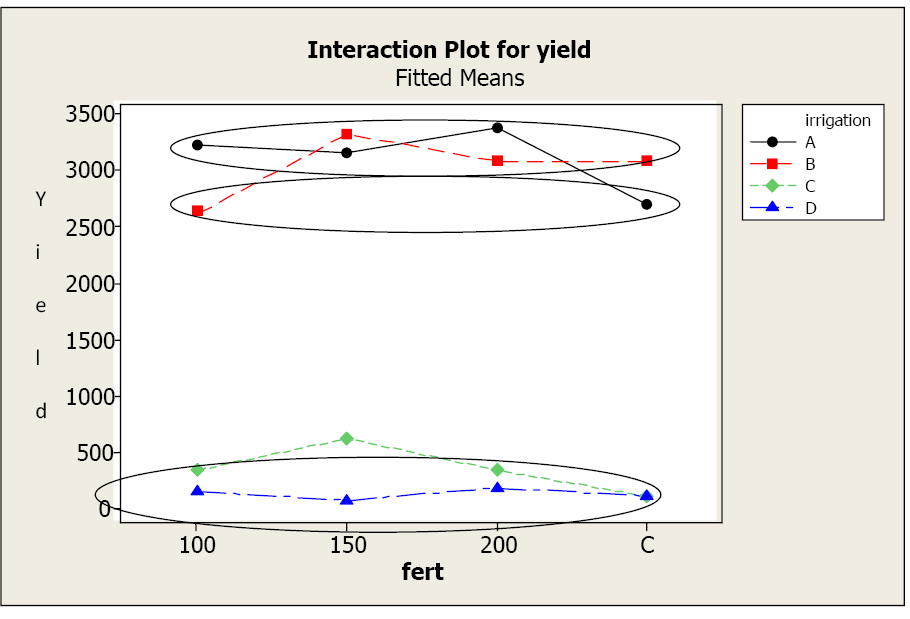
The Grouping Information tells us that while irrigation levels A and B look similar across all levels of fertilizer, only treatments A-100, A-150, A-200, B-control, B-150, and B-200 are statistically similar (upper circle). Treatment B-100 and A-control also result in similar yields (middle circle) and both have significantly lower yields than the first group.
Irrigation levels C and D result in the lowest yields across the fertilizer levels. We again refer to the Grouping Information to identify the differences. There is no significant difference in yield for irrigation level D over any level of fertilizer. Yields for D are also similar to yields for irrigation level C at 100, 200, and control levels for fertilizer (lowest circle). Irrigation level C at 150 level fertilizer results in significantly higher yields than any yield from irrigation level D for any fertilizer level, however, this yield is still significantly smaller than the first group using irrigation levels A and B.
Interpreting Factor Plots
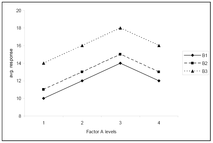
When the interaction term is significant the analysis focuses solely on the treatments, not the main effects. The factor plot and grouping information allow the researcher to identify similarities and differences, along with any trends or patterns. The following series of factor plots illustrate some true average responses in terms of interactions and main effects.
This first plot clearly shows a significant interaction between the factors. The change in response when level B changes, depends on level A.
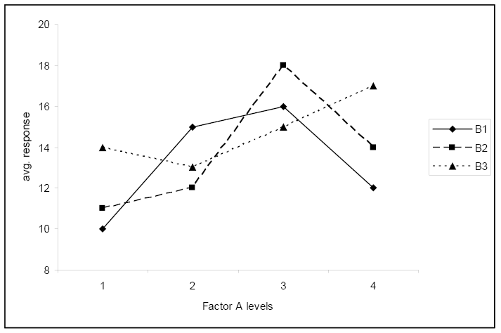
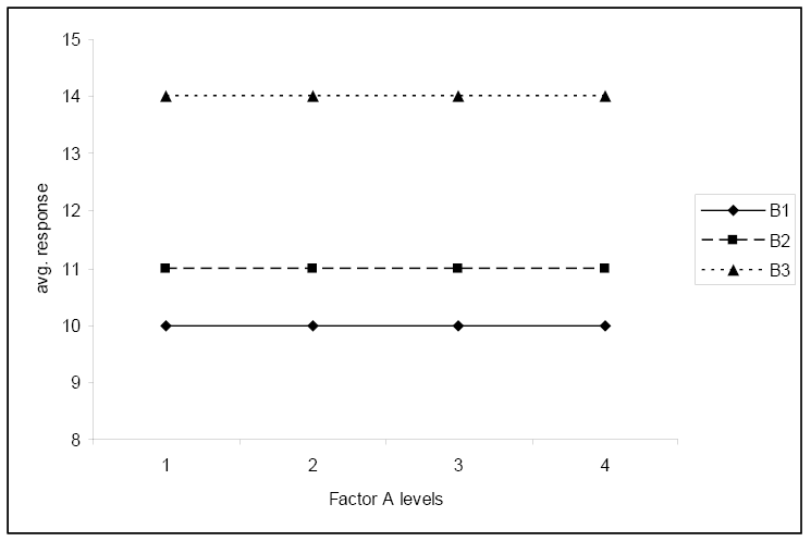
The second plot shows no significant interaction. The change in response for the level of factor A is the same for each level of factor B.
The third plot shows no significant interaction and shows that the average response does not depend on the level of factor A.
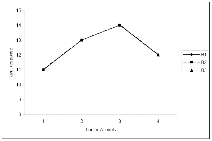
This fourth plot again shows no significant interaction and shows that the average response does not depend on the level of factor B.
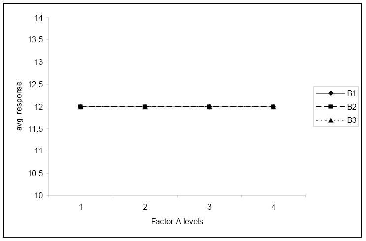
This final plot illustrates no interaction and neither factor has any effect on the response.
Summary
Two-way analysis of variance allows you to examine the effect of two factors simultaneously on the average response. The interaction of these two factors is always the starting point for two-way ANOVA. If the interaction term is significant, then you will ignore the main effects and focus solely on the unique treatments (combinations of the different levels of the two factors). If the interaction term is not significant, then it is appropriate to investigate the presence of the main effect of the response variable separately.
Software Solutions
Minitab


General Linear Model: yield vs. fert, irrigation
|
Factor |
Type |
Levels |
Values |
|||
|
fert |
fixed |
4 |
100, |
150, |
200, |
C |
|
irrigation |
fixed |
4 |
A, |
B, |
C, |
D |
|
Analysis of Variance for Yield, using Adjusted SS for Tests |
||||||
|
Source |
DF |
Seq SS |
Adj SS |
Adj MS |
F |
P |
|
fert |
3 |
1128272 |
1128272 |
376091 |
12.76 |
0.000 |
|
irrigation |
3 |
161776127 |
161776127 |
53925376 |
1830.16 |
0.000 |
|
fert*irrigation |
9 |
2088667 |
2088667 |
232074 |
7.88 |
0.000 |
|
Error |
64 |
1885746 |
1885746 |
29465 |
||
|
Total |
79 |
166878812 |
||||
|
S = 171.653 R-Sq = 98.87% R-Sq(adj) = 98.61% |
||||||
|
Unusual Observations for yield |
|||||||
|
Obs |
yield |
Fit |
SE |
Fit |
Residual |
St |
Resid |
|
4 |
2390.00 |
2700.20 |
76.77 |
-310.20 |
-2.02 |
R |
|
|
28 |
2250.00 |
2646.00 |
76.77 |
-396.00 |
-2.58 |
R |
|
|
35 |
4250.00 |
3327.60 |
76.77 |
922.40 |
6.01 |
R |
|
|
R denotes an observation with a large standardized residual. |
|||||||
|
Grouping Information Using Tukey Method and 95.0% Confidence |
|||||||
|
irrigation |
N |
Mean |
Grouping |
||||
|
A |
20 |
3120.60 |
A |
||||
|
B |
20 |
3040.05 |
A |
||||
|
C |
20 |
352.85 |
B |
||||
|
D |
20 |
129.55 |
C |
||||
|
Means that do not share a letter are significantly different. |
|||||||
|
Grouping Information Using Tukey Method and 95.0% Confidence |
|||||||
|
fert |
N |
Mean |
Grouping |
||||
|
150 |
20 |
1797.90 |
A |
||||
|
200 |
20 |
1749.95 |
A |
||||
|
100 |
20 |
1592.55 |
B |
||||
|
C |
20 |
1502.65 |
B |
||||
|
Means that do not share a letter are significantly different. |
|||||||
|
Grouping Information Using Tukey Method and 95.0% Confidence |
|||||||
|
fert |
irrigation |
N |
Mean |
Grouping |
|||
|
200 |
A |
5 |
3381.00 |
A |
|||
|
150 |
B |
5 |
3327.60 |
A |
|||
|
100 |
A |
5 |
3232.20 |
A |
|||
|
150 |
A |
5 |
3169.00 |
A |
|||
|
200 |
B |
5 |
3097.00 |
A |
|||
|
C |
B |
5 |
3089.60 |
A |
|||
|
C |
A |
5 |
2700.20 |
B |
|||
|
100 |
B |
5 |
2646.00 |
B |
|||
|
150 |
C |
5 |
623.80 |
C |
|||
|
100 |
C |
5 |
340.60 |
C |
D |
||
|
200 |
C |
5 |
338.00 |
C |
D |
||
|
200 |
D |
5 |
183.80 |
D |
|||
|
100 |
D |
5 |
151.40 |
D |
|||
|
C |
D |
5 |
111.80 |
D |
|||
|
C |
C |
5 |
109.00 |
D |
|||
|
150 |
D |
5 |
71.20 |
D |
|||
|
Means that do not share a letter are significantly different. |
|||||||
Excel
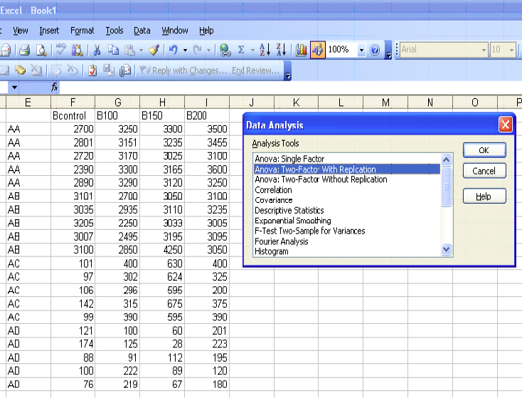
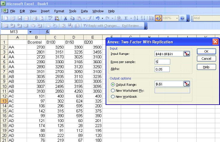
|
Anova: Two-Factor With Replication |
||||||
|
SUMMARY |
Bcontrol |
B100 |
B150 |
B200 |
Total |
|
|
AA |
||||||
|
Count |
5 |
5 |
5 |
5 |
20 |
|
|
Sum |
13501 |
16161 |
15845 |
16905 |
62412 |
|
|
Average |
2700.2 |
3232.2 |
3169 |
3381 |
3120.6 |
|
|
Variance |
35700.2 |
4679.2 |
11167.5 |
40930 |
87716.57 |
|
|
AB |
||||||
|
Count |
5 |
5 |
5 |
5 |
20 |
|
|
Sum |
15448 |
13230 |
16638 |
15485 |
60801 |
|
|
Average |
3089.6 |
2646 |
3327.6 |
3097 |
3040.05 |
|
|
Variance |
5839.8 |
76917.5 |
269901.3 |
7432.5 |
139929.4 |
|
|
AC |
||||||
|
Count |
5 |
5 |
5 |
5 |
20 |
|
|
Sum |
545 |
1703 |
3119 |
1690 |
7057 |
|
|
Average |
109 |
340.6 |
623.8 |
338 |
352.85 |
|
|
Variance |
351.5 |
2525.8 |
1079.7 |
6782.5 |
37326.03 |
|
|
AD |
||||||
|
Count |
5 |
5 |
5 |
5 |
20 |
|
|
Sum |
559 |
757 |
356 |
919 |
2591 |
|
|
Average |
111.8 |
151.4 |
71.2 |
183.8 |
129.55 |
|
|
Variance |
1485.2 |
4135.3 |
997.7 |
1510.7 |
3590.366 |
|
|
Total |
||||||
|
Count |
20 |
20 |
20 |
20 |
||
|
Sum |
30053 |
31851 |
35958 |
34999 |
||
|
Average |
1502.65 |
1592.55 |
1797.9 |
1749.95 |
||
|
Variance |
2069464 |
1977134 |
2317478 |
2359637 |
||
|
ANOVA |
||||||
|
Source of Variation |
SS |
df |
MS |
F |
p-value |
F crit |
|
Sample |
1.62E+08 |
3 |
53925376 |
1830.164 |
5.98E-62 |
2.748191 |
|
Columns |
1128272 |
3 |
376090.7 |
12.76408 |
1.23E-06 |
2.748191 |
|
Interaction |
2088667 |
9 |
232074.2 |
7.876325 |
1.02E-07 |
2.029792 |
|
Within |
1885746 |
64 |
29464.78 |
|||
|
Total |
1.67E+08 |
79 |
||||
